Quantcast
Channel: Microfluidics – COMSOL Blog
Viewing all 31 articles
Browse latest View live

Modeling an Accurate Drug Delivery Device

$
0
0

There are many different routes through which drugs and other medications can be delivered into a patient’s body during treatment. These include topographical ointments, pills, vaporizers, and injection systems, among others. Many of these drug delivery systems require an enormous amount of precision when it comes to the location, timing, concentration, and amount of the drug to be administered. This is where simulation can be a big help, as it can allow for the modeling of each of these aspects of the drug delivery system. When it comes to drug delivery, ensuring that the proper dosage of the drug is administered is key.

Modeling Drug Delivery on the Microfluidic Scale

In a drug dosing system, such as what might be employed by an intravenous (IV) therapy device, the concentration of the drug needed to be delivered into the bloodstream can be incredibly precise. In these systems, the delivery of a drug must be exact; even the smallest difference in amount could potentially inflict harm on the patient. In order to ensure that the correct dosage of a water-soluble drug can precisely and accurately be administered, we can use multiphysics modeling to analyze and optimize the system. In this microfluidic device, we can model the fluid flow of a water droplet as it travels down a capillary tube and comes into contact with a drug concentration. This concept is illustrated in the figure below:

The operating principle of the drug delivery device

Diagram detailing the operating principle of the drug delivery device. The droplet’s color represents the concentration of the drug. As the droplet passes through the section of the capillary surrounded by a permeable membrane, the drug concentration increases (from blue to red).

Because the capillary tube is a cylindrical shape, an axisymmetric geometry can be used to represent the system. A certain section of the capillary tube has its surface coated in a permeable membrane containing a concentrated solution of the drug. When the surface of the droplet comes into contact with the membrane, the drug will diffuse inwards, dispensing the desired dose into the water. The final concentration of the drug within the system will depend on the velocity at which the water droplet is traveling as it passes through the membrane — when the droplet is only in contact with the membrane for a brief period of time, less of the drug will dissolve than if the droplet was touching the membrane for an extended period of time. By varying the velocity of the water droplet, the final concentration of the drug in the droplet can be regulated.

Initially, the water droplet is stationary at the top of the capillary tube. When the droplet is released, it travels down the capillary tube and accelerates to a constant velocity before reaching the permeable membrane. The diffusion coefficient of the drug in the water is 5×10⁻⁹ m2/s. As the surface of the droplet is exposed to the membrane, its velocity is varied between 0.1 and 1 mm/s in order to obtain the final concentration. The velocity field and concentration profiles are quite complex when the droplet first comes into contact with the membrane. Far away from the droplet, the velocity profile corresponds to Poiseuille flow, but near the surface of the droplet, vortices and nonuniformities are present. This is due to the fact that the entire droplet is moving at a fixed velocity of 0.25 mm/s as it passes the membrane. The constant velocity across the width of the capillary causes a significant redistribution of the flow field. This velocity profile occurs 1.5 seconds into the simulation. We can use a simulation to examine the flow field velocity surrounding the droplet and the concentration of the droplet as the drug diffuses into the water. The complex flow field and concentration profile is shown below:

Flow field velocity (small) Drug concentration in the droplet (small)

Velocity of the flow field surrounding the water droplet as it passes into the permeable membrane. Click image to enlarge.

The drug concentration in the droplet as it travels past the edge of the permeable membrane. Click image to enlarge.

Analyzing the Concentration Profile in the Droplet

We can examine the total amount of the drug that has diffused into the droplet as a function of time. In the graph below, we analyze the quantity of the drug in the droplet when the drop is traveling at a speed of 0.1 mm/s. As can be seen in the graph, the drug concentration increases with an s-shaped profile. The steady increase between 3 and 6 seconds corresponds to the time where the droplet’s surface is in contact with the membrane.

Drug concentration increase over time

Additionally, we can measure the total number of moles delivered into the droplet against the droplet’s velocity. As can been seen in the graph below, the number of moles delivered into the droplet is approximately inversely proportional to the velocity of the droplet. Therefore, we can vary the amount of drug that is allowed to diffuse into the droplet by altering the time it takes for the drug to pass entirely through the membrane. With simulation, we are able to precisely and accurately anticipate the exact velocity needed in order to achieve a certain drug dosage. This system is accurate down to the picomole, and using simulation we can find the optimal velocity and time in order to administer a desired drug concentration.

Drug concentration vs. droplet velocity

Additional Resources


Modeling Electroosmotic Flow and the Electrical Double Layer

$
0
0

Microfluidic devices are so small that the micropumps and micromixers that control and mix the fluid inside the device cannot involve any moving components. Instead, they must take advantage of electroosmotic flow. Here, I will describe the concept of electroosmosis and the electrical double layer (EDL), and how to model these in COMSOL, walking you through two example models.

Microfluidic Devices Require Pumps and Mixers without Moving Parts

Microfluidic lab-on-a-chip systems have played a major role in recent years in shrinking the size of conventional lab-scale chemical and biological analyses to a chip-format that is millimeters to a few centimeters in size. These devices are often referred to as micro-total-analysis-systems (μTAS) and have profound applications in medical diagnostics, drug testing and delivery, forensic analysis, DNA analysis, and even immunoassays and toxicity monitoring. These devices offer many advantages such as point-of-care testing (POCT) and diagnostics due to their extremely small device size. The fact that they require a smaller volume of fluids is suitable for situations where samples are not available in large volumes or when reagents are expensive. These devices can also process multiple samples at once (referred to as parallel processing) and have low power requirement.

On-board mixing and control of fluid is important in a typical lab-on-a-chip system and often these systems require micropumps to control the fluid flow inside the channels and micromixers to accelerate the mixing process. The size of the fluid channels in these microchips typically varies between 1 µm and 500 µm. At these length scales, it is not practical to use any moving parts to build the pumps and mixers. Devices without moving parts are also more reliable. So how do you activate the flow without any moving parts? The answer is: Electroosmosis.

What “Electroosmosis” Means

In the field of microfluidics, the flow is often driven by an electric field. By definition, electroosmosis refers to the motion of a liquid induced by an applied potential across a microchannel. Driving the flow with an electric field allows for the fabrication of pumps and mixers without moving parts.

What drives the electroosmotic flow?

To get a better understanding of how the flow is driven by an electric field, we first have to understand what happens very close to the walls inside the microchannels, at the fluid-solid interface. The majority of lab-on-a-chip devices are made out of silicon glass. When in contact with the fluid (it can be water or any buffered solution), the glass surface participates in acid-base reactions and ion exchange — we will refer to this complex process as surface chemistry. Because of surface chemistry, the glass surface acquires a negative density charge. The concept of electrical double layer (EDL) has been introduced as a continuum description of this surface chemistry at the walls. It reflects an unequal distribution of charges (ions) at the fluid-solid interface and consists of two layers surrounding the object:

  1. The first layer, known as the surface charge layer, is made of ions absorbed in the surface due to chemical reactions (negative charges in this case).
  2. The second layer, known as the diffusive layer, is made of free ions attracted to the surface due to the influence of electric attraction and thermal motion. This second layer screens the surface charge and its net charge is equal to the surface charge, but has the opposite polarity.

Electrical double layer showing the unequal distribution of ions and the potential in the EDL versus in the electroneutral bulk
Electrical double layer (EDL).

The EDL structure is summarized in the figure above, showing the distribution of ions as a function of the distance to the glass wall, as well as the potential (blue line on top) in the EDL versus a point in the electroneutral bulk. If we take a closer look at the diffusive layer, we notice that it can be further split into two parts that are separated by a slipping plane. This plane separates the immobile fluid on the left (attached to the surface), from the fluid that is free to move under the influence of tangential stress. An electric field can then be used to induce the motion of the net charge in the EDL due to the Coulomb force. Further away from the wall is the third layer, the electroneutral bulk.

Since it’s difficult to make any kind of measurement in microfluidic channels without disrupting the flow, these chips are often analyzed from a computational point of view. How can we model this using simulation software?

Modeling of the Electrical Double Layer (EDL)

Three physics are involved in this problem:

  1. The electrostatics physics contains the equations, boundary conditions, and space charges for solving for the electric potential. The electric field is recovered from the gradients of the potential field (E=-\nabla V). The space charge is obtained by summing up the contribution of the anions and the cations. The concentration of these ions is computed by the Transport of Diluted Species interface.
  2. The Transport of Diluted Species interface solves for the mass transport of diluted species in mixtures, solving for the species concentrations. It simulates chemical species transport through diffusion (Fick’s law), migration (when coupled to an electric field. In this case, the electrical field is computed by the Electrostatics interface), and convection (when coupled to fluid flow. Here, the fluid flow is computed by the Laminar flow interface.)
  3. The Laminar flow interface has the equations, boundary conditions, and volume forces for modeling freely moving fluids using the Navier-Stokes equations, solving for the velocity field and the pressure. The volume force, \rho_{e} E, where \rho_{e} is the electric charge density, is computed by the Electrostatics interface.

The thickness of the EDL is generally around a few nanometers and the concentration of the ions varies exponentially close to the wall. Since the thickness of the EDL is so small, it can be advantageous to use an approximation in this region. COMSOL includes an electroosmotic velocity boundary condition that ignores the flow field between the wall and the slipping plane, and analytically computes the velocity at the wall based on the zeta potential using the Helmholtz-Smoluchowski relation:

\textbf{u}=\frac{\epsilon_{W} \zeta_{0}}{\eta} \nabla_{T} V

The resulting models will have significantly lower computational requirements. This is a very useful approach for many practical engineering applications.

Therefore, we recommend that you first calculate the Debye length, i.e. the length of the EDL, before you set up the model using COMSOL Multiphysics. If this length is much smaller than your geometrical length scale, use the electroosmotic velocity boundary condition. If not, use the traditional no-slip velocity wall boundary condition and resolve the flow in the EDL. Remember that concentration varies exponentially with potential in the double layers; a fine boundary layer mesh is necessary to resolve the abrupt change in the double layers if the electroosmotic velocity boundary condition is not used.

In the next section I will show you two examples where this applies. The first example is of a micropump that is resolved in the whole geometry, including the EDL. The second example, a micromixer, uses the electroosmotic velocity boundary condition.

Applications

Example 1: Micropumps

In this example, the top and bottom walls of the microchannel (length 60 nm, height 10 nm) are negatively charged (-0.02 C/m^{2}) and electrodes are used at the inlet (left boundary, 6 mV) and outlet (right boundary, 0 V) to drive the flow. The resulting electric potential, space charge distribution, and velocity field are shown below:

Plot showing the electrical potential of the microchannel computed by the electrostatics physics
Plot visualizing the electric potential computed by the electrostatics physics.

The contribution of the anions and cations in the microchannel resulting in the net space charge
Plot depicting the net space charge, i.e. the contribution of the anions and the cations. The positive net charge screens the negatively charged wall.

Velocity plot depicting the movement of the net charge in the EDL
Velocity plot showing the motion of the net charge in the EDL due to the Coulomb force. This model is available upon request from Tech Support.

In order to introduce the next example, the micromixer, let’s first see what happens when sections of the top and bottom glass walls (shown in blue in the next plot) are positively charged (0.06 C/m^{2}) instead of negatively charged:

Geometry with positively charged sections instead of negatively charged sections

The results for the electric potential, space charge, and velocity field follow:

Electric potential in the EDL geometry with positively charged sections
Space charge in the EDL geometry with positively charged sections
Electroosmotic velocity in the EDL geometry with positively charged sections

While the space charge is positive around negatively charged walls, it is negative around the positively charged portions. The inversion of the space charge leads to an opposite electroosmotic velocity close to the wall. This opposite near-wall velocity leads to the introduction of a swirl in the channel (as seen in the streamline patterns), which could be used to mix different chemical species.

Example 2: Micromixers

At the microscale, flow is usually a highly ordered laminar flow, and the lack of turbulence makes diffusion the primary mechanism for mixing. While diffusional mixing of small molecules (and therefore of rapidly diffusing species) can occur in a matter of seconds over distances of tens of micrometers, mixing of larger molecules such as peptides, proteins, and high molecular-weight nucleic acids can require equilibration times from minutes to hours over comparable distances. Such delays are impractically long for many chemical analyses. These problems have led to an intense search for more efficient mixers for microfluidic systems. In the following example, the walls are negatively charged, as in the micropump example we just went over, and electrodes are used at the inlet (left boundary) and outlet (right boundary) to drive the flow. To introduce some mixing, four additional electrodes are placed on the walls of the mixing chamber. These four electrodes induce a fluctuating electroosmotic velocity at the wall:

Plot showing how the mixer functions

Plot exemplifying how the mixer operates. Two fluids with different concentrations are
used at the inlet to study the mixing process.

Plot of the electroosmotic flow showing how the mixer works

When the electric field is not applied, the flow is laminar and the diffusion coefficient is very small, so the two fluids are well separated at the outlet.

The mixer when an alternating electric field is applied

When the alternating electric field is applied, the mixing increases considerably, owing to the alternating swirls in the flow.

Concluding Thoughts and Next Steps

This blog post briefly described electroosmotic flow and the concept of the electrical double layer. You also learned how to model this type of problem within the COMSOL environment. If you want even more information about the Electroosmotic Micromixer model, you can download the model and model documentation from our Model Gallery. You can get a general overview of COMSOL’s microfluidics modeling capabilities here, or contact us for more in-depth information on how you can use COMSOL Multiphysics to model a variety of applications.

Finally, don’t forget that COMSOL is a multiphysics software, allowing you to couple the physics seen in this model to other physics. Adding the particle tracing physics, for instance, would allow you to model electrokinetic phenomena such as electrophoresis and dielectrophoresis.

Thermometer Calibration: When Experimentation Falls Short

$
0
0

The International Temperature Scale of 1990 (ITS-90) is the industry calibration standard for measuring temperatures throughout the world. The National Physical Laboratory (NPL) works to establish and maintain the ITS-90 through experiments, most notably, thermometer calibration. To better understand and overcome the shortcomings of the experimental process, Jonathan Pearce, at the UK’s National Physics Laboratory, turned to simulation. His results yielded fascinating results about the microscopic behavior of the liquid-solid interface during the freezing process.

National Physical Laboratory’s Work on Thermometer Calibration

The Temperature and Humidity department at the National Physical Laboratory, of which Jonathan Pearce is a team member, works to enhance the accuracy of temperature measurements to preserve and improve the ITS-90. Specified in the ITS-90, the NPL uses standard platinum resistance thermometers, widely accepted as the most accurate thermometers. Even so, when calibrating these thermometers, there is a level of uncertainty involved. For the model used by Jonathon Pearce (measuring the freezing point of zinc), the uncertainty range is 1 millikelvin.

Standard platinum resistance thermometer designed by the National Physical Laboratory
Cross section of a standard platinum resistance thermometer (SPRT)used for calibration. Image courtesy: The National Physical Laboratory.

Optimizing Experimentation Through Simulation

Although the platinum resistance thermometer is the most accurate device used for temperature calibration, the uncertainty of 1 millikelvin could stand to be improved. This uncertainty led Pearce to turn to simulation, to better understand the freezing process at a microscopic level and to identify what the sensors were measuring. Working with Surrey University student Matthew Large, Pearce used COMSOL Multiphysics to delve into the inner workings of the freezing process. The results found that the freezing process is not planar; it is not smooth at the liquid-solid interface. As the liquid begins to freeze into a solid, ripples form at the interface and turn into cells, protruding outwards unevenly (as seen in the image below). This phenomenon could not be predicted or measured using experimentation, however, through simulation, they were able to obtain valuable information in order to redesign the device for more accurate thermometer calibration experiments.

Thermometer calibration using simulation to model the liquid-solid interface
Cells protruding outwards at the liquid-solid interface.

Further Reading… and Viewing

Red Blood Cell Separation from a Flow Channel

$
0
0

Before conducting certain blood sample analyses, researchers need to separate the red blood cell particles from the blood plasma. Using lab-on-a-chip (LOC) technology, red blood cell separation can be achieved via magnetophoresis, i.e. motion induced by magnetic fields. Since the magnetic permeability of the particles is different from the blood plasma, their trajectory can be controlled within the flow channel of the LOC device and thereby separated out from the fluid.

Blood Plasma and Red Blood Cells

Whole blood consists of red and white blood cells, as well as platelets suspended in a liquid referred to as blood plasma. According to the American Red Cross, plasma is 92% water and makes up 55% of blood volume. The permeability of blood plasma is equal to 1.

Red blood cells make up slightly lower blood volume than blood plasma — about 45% of whole blood. As you probably already know, these types of blood cells contain hemoglobin, which in turn consists of iron that helps transport oxygen throughout the body. The permeability of red blood cells is slightly less than 1, (1 – 3.9e-6). Or to put it in words, red blood cell particles are diamagnetic.

Red Blood Cell Separation via Magnetophoresis in LOCs

Lab-on-a-chip devices (LOCs) are very small (picture an area in the millimeter-centimeter range) microfluidic devices consisting of flow channels that perform one or more lab functions on a single chip. LOCs are frequently used in medicine and research for analyzing samples of blood, thanks to the reduced risk of sample contamination made possible by the ability to collect and study very small samples.

Due to their aforementioned magnetic properties, red blood cells may be separated from the plasma via a magnetophoretic approach. If we were to subject the LOC channel to a magnetophoretic force, we could control where the red blood cells and the plasma go within the channels. In other words, because the red blood cells have different permeability, they can be separated from the flow channel.

Suppose we have an LOC containing blood plasma (in this case that’s considered the background fluid) and red blood cell particles in a channel that splits into three branches, or outlets (see image below). The drag force of the background fluid pushes the particles forward along the flow channel. Now suppose we have a permanent magnet on each side of the channel, as such:

Lab-on-a-chip with two neodymium permanent magnets and a flow channel
LOC: Two neodymium permanent magnets and a flow
channel with three outlets and an array of soft iron patches.

The magnetophoretic force of the magnets will push the blood cell particles inward. Combined, the drag force and the magnetophoretic force will simultaneously push the particles toward the center and through the main channel, bypassing the two channel branches. Meanwhile, the blood plasma, which, as mentioned above, has a permeability of 1, is not affected by the magnetic field and simply travels along in the direction of the drag force. This ultimately leads one third of the plasma to flow through each of the channels, while all of the red blood cells are concentrated in the center channel — providing us with a high enough concentration to study.

My colleague John Dunec has created a multiphysics simulation to illustrate the concept:

Red blood cell separation via magnetophoresis
Red blood cell separation: An LOC device, zooming in on the flow channels. The red blood
cell particles travel in the center channel.

The above simulation was created with COMSOL Multiphysics together with the AC/DC, Microfluidics, and Particle Tracing modules. A tutorial on how to run this on your own can be found in the section below.

Further Reading

Buoyancy-Driven μPCR for DNA Amplification

$
0
0

DNA is a complex molecule that contains instructions for life and often referred to as a “digital fingerprint” or code telling a cell what to do. DNA is often the only means for accurate testing and identification of biomolecules, cells, or even an entire person during forensic investigations. The need to be able to test for DNA, as quickly as possible, and even at the site where the sample is taken, is becoming more and more important.

Polymerase Chain Reaction (PCR) and DNA Amplification

The more DNA one has in a sample, the easier it is to identify and diagnose. In many situations, such as old crime scenes or large ecological systems with dilute samples, you want to amplify the amount of available DNA before testing for it. One technique that is most effective in amplifying DNA and making it useful in medical diagnostic, chemical, and biological analysis is Polymerase Chain Reaction, commonly known as PCR. It is also referred as a DNA amplification technique. Further, there has been great interest in recent years in developing portable PCR-based micro total analysis systems (μTAS; also known as lab-on-a-chip systems) for point-of-care applications.

One strategy that seems very promising is natural convection-based PCR. In this strategy, many copies of a DNA template can be made by cycling between hot and cold regions within a microreactor via a buoyancy-driven flow. The multiphysics nature of this strategy makes it a perfect candidate for simulations with COMSOL software.

A COMSOL model can provide more quantitative understanding of the dynamics and kinetics involved in the process that will be very useful in designing and developing efficient μTAS. Here, I will show you a model that was developed to study the spatio-temporal variation of the concentrations of single-stranded (ssDNA), double-stranded (dsDNA), and primer-annealed (aDNA) DNA components during natural convection-based PCR. The model is available for download from the Model Gallery.

The driving mechanism for the fluid motion is the temperature-induced density differences that results in buoyancy flow. This approach eliminates the need for an external driving mechanism as the difference between the temperatures is sufficient to circulate the PCR mixture and amplify DNA in a closed loop, as shown below.
Schematic of buoyancy-driven PCR
Schematic of buoyancy-driven PCR.

In general, a PCR mixture consists of a DNA template, primers, nucleotides, and the enzymes (Taq polymerase, the most widely used amplifying enzyme). The mixture is repeatedly cycled between three temperature zones:

  • Denaturing zone (95°C): Double-stranded DNA template is separated into two single strands.
  • Annealing zone (55°C): Primers bind to the ends of the single-stranded DNA.
  • Extension zone (72°C): A complement to each of the annealed single strands is created by enzyme resulting in two new copies of double strands DNA template. Repeating the above process results in an exponential increase in DNA concentration.

Developing a Bouyancy-Driven PCR Model

In the figure above, you can see the 2D model geometry of the buoyancy-driven PCR. A dilute PCR mixture fills the channel with an impermeable wall. The right and left boundaries of the channel are maintained at 95°C and 55°C, respectively. The upper and lower boundaries are insulated. The temperature gradient produces variation in the density of fluid that drives the buoyant flow. The model uses temperature-dependent properties for water. The predefined Non-Isothermal Flow/Conjugate Heat Transfer interface available in the CFD Module or the Heat Transfer Module is used to model coupled heat transfer and the fluid flow physics.

The DNA components are generated and consumed by the temperature-dependent chemical reactions as proposed in “Polymerase chain reaction in natural convection systems: A convection–reaction-diffusion model” by E. Yariv, G. Ben-Dov, and K. D. Dorfman. A simplified first-order reaction mechanism (given below) illustrates the PCR process that is used in this model. The rates of change in the concentration of DNA components were determined from the stoichiometric balances.

\mathit{dsDNA}\xrightarrow{k_d}2\mathit{ssDNA} Denaturation (95°C)
\mathit{ssDNA}\xrightarrow{k_a}\mathit{aDNA} Annealing (55°C)
\mathit{aDNA}\xrightarrow{k_e}\mathit{dsDNA} Extension (72°C)

These reaction rates constants were spatially modulated using the below Gaussian mapping function. This is done in order to localize each reaction in its respective temperature zone.

f_i=\exp{\left(-{\frac{{(T-{T_i})^2}}{2{\sigma^2}}}\right)}

Here, \sigma (=1°C) is the standard deviation of the reaction rate with respect to temperature and T_i is the ideal temperature for denaturation (95°C), annealing (55°C), and extension (72°C) reaction (at which the function is maximized). The multicomponent mass transfer of DNA components in the channel is governed by the convection and diffusion equation, and is modeled using the Transport of Dilute Species interface from the Chemical Reaction Engineering Module.

A step-wise approach is used to solve the coupled system of heat transfer, fluid flow, and mass transfer. Non-Isothermal Flow physics is solved at steady state, and the velocity field that is obtained is used in the mass transfer equation to obtain time varying concentrations of DNA components.

Modeling Results

Below, we can see the steady-state velocity profile and temperature contours across the channel. We can note that a large convective cell occupies the channel and the fluid flows along the boundaries and is faster at the vertical walls where the temperature variations are highest.
Plot depicting the temperature Distribution and Velocity Magnitude
Temperature distribution and velocity magnitude.

Next, we can look at the reaction rates for denaturation, annealing, and extension reactions after 120 seconds. It is clear that these reactions are localized around 95°C, 55°C, and 72°C respectively. It will be interesting to see the variation of these reaction rates with respect to time.
Reaction rates for denaturation, annealing, and extension reactions
Reaction rates for denaturation, annealing, and extension reactions after 120 s.

Initially only denaturation is taking place in the channel, but after a certain amount of time, annealing and extension effects are also visible.

Variation of reaction rates for denaturation, annealing, and extension with time
Variation of reaction rates for denaturation, annealing, and extension with time.

Interesting results are obtained when the concentrations of DNA components are monitored. In the plot below, you can see the concentration profile of DNA components for a simulation time of 120s.
Concentration Profile of DNA Components
Concentration Profile of DNA Components.

It is evident that the concentration of the double-strand DNA template (dsDNA) initially decreases due to denaturation, but later on exponentially increases due to the amplification effect in the extension region. It is common to use the doubling time in order to quantitatively characterize PCR efficiency. The doubling time is the time required to double the concentration of initial double-strand DNA template (dsDNA) used in the mixture. From the concentration plot, the doubling time is around 60 seconds, which is of the same order of magnitude as given in the aforementioned literature. In general, the doubling time of a laboratory scale conventional PCR system is around two minutes.

Conclusion and Next Steps

This blog post briefly described a multiphysics model for DNA amplification by PCR in a buoyancy-driven flow. It can be used to understand the amplification rates as a function of the device parameters, which will be very useful in device design and optimization. More realistic reaction data can be brought on-board, and geometric parameters can be varied. In general, it is possible to extend the scope of this model using the powerful and flexible user interfaces of the Heat Transfer, CFD, and Chemical Reaction Engineering modules.

Model Download

Tesla Microvalve Model as a Topological Optimization Example

$
0
0

Topological optimization is routinely used in the design and refinement of microfluidics devices. The process also comes in handy for modeling a Tesla microvalve.

What Is a Tesla Microvalve?

The Tesla microvalve is a valve that allows fluid to flow freely in one direction but not in the reverse. This valve is one of the many inventions designed by the famous late Nikola Tesla. In recognition of Tesla’s 158th birthday anniversary, my colleague Fanny Littmarck wrote about his life and many contributions to science and engineering. She did not mention the microvalve, however. Perhaps because it is often overshadowed by his electrical inventions.

What makes this valve so fascinating is the fact that it has no moving mechanical parts. This design greatly reduces the risk of wearing out or breaking down. You may be asking yourself, “Well, how does the valve stop fluid without any moving parts?” Interestingly enough, the valve’s fixed geometry inhibits reverse flow through the utilization of friction forces. Thanks to the design, the fluid itself becomes the inhibiting force.

The geometry of a Tesla microvalve.
Tesla microvalve schematic from Tesla’s “Valvular conduit” patent. Inlet on the right end, outlet on the left end.

To achieve this effect, the microvalve design can be optimized by dispersing a distinct amount of material within the modeling domain.

Optimizing the Tesla Microvalve Design

When modeling microfluidic devices, topological optimization is often used to refine the model. The Topological Optimization of a Tesla Microvalve model serves as an exceptional example of how you can do just that, using COMSOL Multiphysics together with the Microfluidics Module. In the case of a Tesla microvalve, you can gauge the effectiveness of your design by obtaining the ratio of the pressure drop between the inlet and outlet for both forward and reverse flows.

By checking out the model, you will learn how to work with two laminar flow interfaces, one for the forward flow and another for the reverse. Additionally, you will see how two instances of the Navier-Stokes equations are computed for the same flow types.

In this example, the optimized design has a triangular-shaped material placed close to the outlet, allowing the forward flow to bend around it. This results in a low pressure drop between the inlet and outlet.

Design shows the forward flow interface within the topological optimization model.
Forward flow in the optimized design after 150 iterations.

In the reverse direction, the flow meets the triangular material’s flat edge, causing the backward flow’s velocity to reroute upwards and downwards toward the device’s walls. The redirected flow’s path is further impeded as it is forced toward additional obstacles.

Optimized design depicting the reverse flow interface of the model.
Reverse flow in the optimized design.

Using a global evaluation, the ratio of the pressure drop between the forward and reverse flow is computed. The value is approximately 1.85.

Model Download

Dielectrophoretic Separation

$
0
0

How can you use an electric field to control the movement of electrically neutral particles? This may sound impossible, but in this blog entry, we will see that the phenomenon of dielectrophoresis (DEP) can do the trick. We will learn how DEP can be applied to particle separation and demonstrate a very easy-to-use biomedical simulation app that is created with the Application Builder and run with COMSOL Server™.

Forces on a Particle in an Inhomogeneous Static Electric Field

The dielectrophoretic effect will show up in both DC and AC fields. Let’s first look at the DC case.

Consider a dielectric particle immersed in a fluid. Furthermore, assume that there is an external static (DC) electric field applied to the fluid-particle system. The particle will in this case always be pulled from a region of weak electric field to a region of strong electric field, provided the permittivity of the particle is higher than that of the surrounding fluid. If the permittivity of the particle is lower than the surrounding fluid, then the opposite is true; the particle is drawn to a region of weak electric field. These effects are known as positive dielectrophoresis (pDEP) and negative dielectrophoresis (nDEP), respectively.

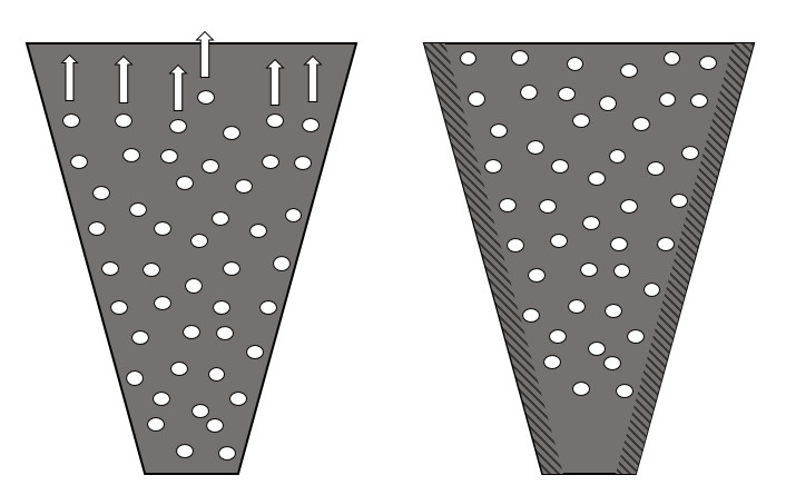
The pictures below illustrate these two cases with a few important quantities visualized:

  • Electric field
  • Maxwell stress tensor (surface force density)
  • Surface charge density

An illustration depicting positive dielectrophoresis.
An illustration of positive dielectrophoresis (pDEP), where the particle permittivity is higher than that of the surrounding fluid \epsilon_p > \epsilon_f. At the surface of the particle, the induced surface charge is color-coded with red representing a positive charge and green a negative charge. Yellow represents a neutral charge.

An image showing negative dielectrophoresis.
An illustration of negative dielectrophoresis (nDEP), where the particle permittivity is lower than that of the surrounding fluid \epsilon_p < \epsilon_f.

The Maxwell stress tensor represents the local force field on the surface of the particle. For this stress tensor to be representative of what forces are acting on the particle, the fluid needs to be “simple” in that it shouldn’t behave too weirdly either mechanically or electrically. Assuming the fluid is simple, we can see from the above illustrations that the net force on the particle appears to be in opposite directions between the two cases of pDEP and nDEP. Integrating the surface forces will indeed show that this is the case.

It turns out that if we shrink the particle and look at the infinitesimal case of a very small particle acting like a dipole in a fluid, then the net force is a function of the gradient of the square of the electric field.

Why is the net force behaving like this? To understand this, let’s look at what happens at a point on the surface of the particle. At such a point, the magnitude of the electric surface force density, f, is a function of charge times electric field:

(1)

f \propto \rho E

where \rho is the induced polarization charges. (Let’s ignore for the moment that some quantities are vectors and make a purely phenomenological argument by just looking at magnitudes and proportionality.)

The induced polarization charges are proportional to the electric field:

(2)

\rho \propto \epsilon E

Combining these two, we get:

(3)

f \propto \rho E = \epsilon E^2

But this is just the local surface force density at one point at the surface. In order to get a net force from all these surface force contributions at the various points on the surface, there needs to be a difference in force magnitude between one side of the particle and the other. This is why the net force, \bf{F}, is proportional to the gradient of the square of the electric field norm:

(4)

\mathbf{F} \propto \epsilon \nabla |\mathbf{E}|^2

In the above derivation, we have taken some shortcuts. For example, what is the permittivity in this relationship? Is it that of the particle or that of the fluid or maybe the difference of the two? What about the shape of the particle? Is there a shape factor?

Let’s now address some of these questions.

Force on a Spherical Particle

In a more stringent derivation, we instead use the vector-valued relationship for the force on an electric dipole:

(5)

\mathbf{F} = \mathbf{P} \cdot \nabla \mathbf{E}

where \bf{P} is the electric dipole moment of the particle.

To get the force for different particles, we simply insert various expressions for the electric dipole moment. In this expression, we can also see that if the electric field is uniform, we get no force (since the particle is small, its dipole moment is considered a constant). For a spherical dielectric particle with a (small) radius r_p in an electric field, the dipole moment is:

(6)

\mathbf{P} = 4 \pi r_p^3 k \mathbf{E}

where k is a parameter that depends on the the permittivity of the particle and the surrounding fluid. The factor 4 \pi r_p^3 can be seen as a shape factor.

Combining these, we get:

(7)

\mathbf{F} = 4 \pi r_p^3 k \mathbf{E} \cdot \nabla\mathbf{E} = 2 \pi r_p^3 k \nabla |\mathbf{E}|^2

This again shows the dependency on the gradient of the square of the magnitude of the electric field.

Forces on a Particle in a Time-Varying Electric Field

If the electric field is time-varying (AC), the situation is a bit more complicated. Let’s also assume that there are losses that are represented by an electric conductivity, \sigma. The dielectrophoretic net force, \bf{F}, on a spherical particle turns out to be:

(8)

\mathbf{F} = 2 \pi r^3_p k \nabla |\mathbf{E}_{\textrm{rms}}|^2

where

(9)

k = \epsilon_0 \Re\{ \epsilon_f \} \Re \left\{ \frac{\epsilon_p -\epsilon_f}{\epsilon_p + 2 \epsilon_f} \right\}

and

(10)

\epsilon = \epsilon_{\textrm{real}} -j \frac{\sigma}{2 \pi \nu}

is the complex-valued permittivity. The subscripts p and f represent the particle and the fluid, respectively. The radius of the particle is r_p and \bf{E}_{\textrm{rms}} is the root-mean-square of the electric field. The frequency of the AC field is \nu.

From this expression, we can get the force for the electrostatic case by setting \sigma = 0. (We cannot take the limit when the frequency goes to zero, since the conductivity has no meaning in electrostatics.)

In the expression for the DEP force, we can see that indeed the difference in permittivity between the fluid and the particle plays an important role. If the sign of this difference switches, then the force direction is flipped. The factor k involving the difference and sum of permittivity values is known as the complex Clausius-Mossotti function and you can read more about it here. This function encodes the frequency dependency of the DEP force.

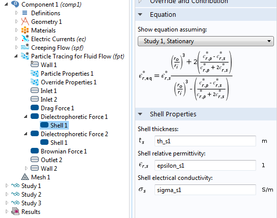
If the particles are not spherical but, say, ellipsoidal, then you use another proportionality factor. There are also well-known DEP force expressions for the case where the particle has one or more thin outer shells with different permittivity values, such as in the case of biological cells. The simulation app presented below includes the permittivity of the cell membrane, which is represented as a shell.

The settings window shows DEP permittivity for a dielectric shell.
The settings window for the effective DEP permittivity of a dielectric shell.

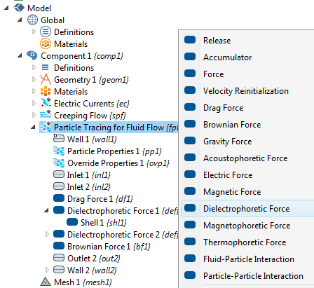
There may be other forces acting on the particles, such as fluid drag force, gravitation, Brownian motion force, and electrostatic force. The simulation app shown below includes force contributions from drag, Brownian motion, and DEP. In the Particle Tracing Module, a range of possible particle forces are available as built-in options and we don’t need to be bothered with typing in lengthy force expressions. The figure below shows the available forces in the Particle Tracing for Fluid Flow interface.

A screenshot highlighting different particle force options.
The different particle force options in the Particle Tracing for Fluid Flow interface.

Dielectrophoretic Separation of Particles

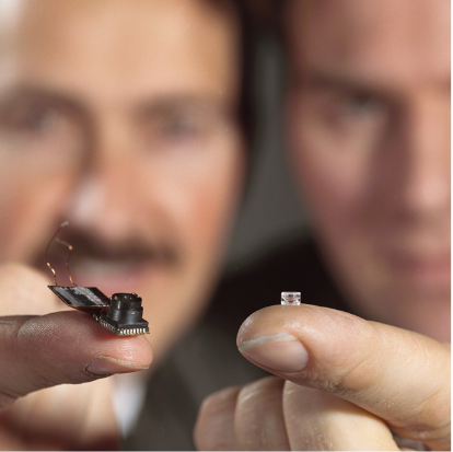
Medical analysis and diagnostics on smartphones is about to undergo rapid growth. We can imagine that, in the future, a smartphone can work in conjunction with a piece of hardware that can sample and analyze blood.

Let’s envision a case where this type of analysis can be divided into three steps:

  1. Extract blood using the hardware, which attaches directly to your smartphone, and compute mean platelet and red blood cell diameter.
  2. Compute the efficiency of separation of the red blood cells and platelets. This efficiency needs to be high in order to perform further diagnostics on the isolated red blood cells.
  3. Use the computed optimum separation conditions to isolate the red blood cells using the hardware attached to your smartphone.

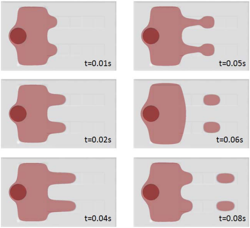
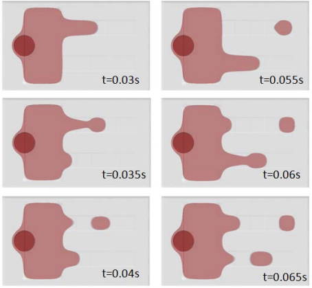
The COMSOL Multiphysics simulation app focuses on Step 2 of the overall analysis process above. By exploiting the fact that blood platelets are the smallest cells in blood and have different permittivity and conductivity than red blood cells, it is possible to use DEP for size-based fractionation of blood; in other words, to separate red blood cells from platelets.

Red blood cells are the most common type of blood cell and the vertebrate organism’s principal means of delivering oxygen (O2) to the body tissues via the blood flow through the circulatory system. Platelets, also called thrombocytes, are blood cells whose function is to stop bleeding.

Using the Application Builder, we created an app that demonstrates the continuous separation of platelets from red blood cells (RBCs) using the Dielectrophoretic Force feature available in the Particle Tracing for Fluid Flow interface. (The app also requires one of the following: the CFD Module, Microfluidics Module, or Subsurface Flow Module and either the MEMS Module or AC/DC Module.)

The app is based on a lab-on-a-chip (LOC) device described in detail in a paper by N. Piacentini et al., “Separation of platelets from other blood cells in continuous-flow by dielectrophoresis field-flow-fractionation”, from Biomicrofluidics, vol. 5, 034122, 2011.

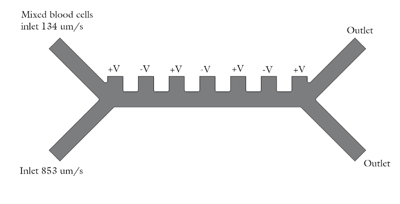
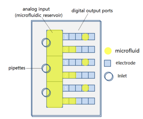
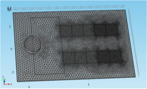
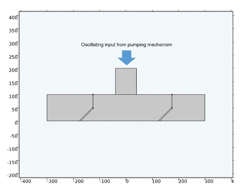
The device consists of two inlets, two outlets, and a separation region. In the separation region, there is an arrangement of electrodes of alternating polarity that controls the particle trajectories. The electrodes create the nonuniform electric field needed for utilizing the dielectrophoretic effect. The figure below shows the geometry of the model.

A schematic of the geometry of the particle separation simulation app.
The geometry used in the particle separation simulation app.

The inlet velocity for the lower inlet is significantly higher (853 μm/s) than the upper inlet (154 μm/s) in order to focus all the injected particles toward the upper outlet.

The app is built on a model that uses the following physics interfaces:

  1. Creeping Flow (Microfluidics Module) to model the fluid flow.
  2. Electric Currents (AC/DC or MEMS Module) to model the electric field in the microchannel.
  3. Particle Tracing for Fluid Flow (Particle Tracing Module) to compute the trajectories of RBCs and platelets under the influence of drag and dielectrophoretic forces and subjected to Brownian motion.

Three studies are used in the underlying model:

  1. Study 1 solves for the steady-state fluid dynamics and frequency domain (AC) electric potential with a frequency of 100 kHz.
  2. Study 2 uses a Time Dependent study step, which utilizes the solution from Study 1 and estimates the particle trajectories without the dielectrophoretic force. In this study, all particles (platelets and RBCs) are focused to the same outlet.
  3. Study 3 is a second Time Dependent study that includes the effect of the dielectrophoretic force.

You can download the model that the app was based on here.

A Biomedical Simulation App

To create the simulation app, we used the Application Builder, which is included in COMSOL Multiphysics® version 5.0 for the Windows® operating system.

The figure below shows the app as it looks like when first started. In this case, we have connected to a COMSOL Server™ installation in order to run the COMSOL Multiphysics app in a standard web browser.

A biomedical simulation app.
A biomedical simulation app running in a standard web browser.

The app lets the user enter quantities, such as the frequency of the electric field and the applied voltage. The results include a scalar value for the fraction of red blood cells separated. In addition, three different visualizations are available in a tabbed window: the blood cell and platelet distribution, the electric potential, and the velocity field for the fluid flow.

The figures below show visualizations of the electric potential and the flow field.

A screenshot showing the microfluidic channel's instantaneous electric potential.
Screenshot showing the instantaneous electric potential in the microfluidic channel.
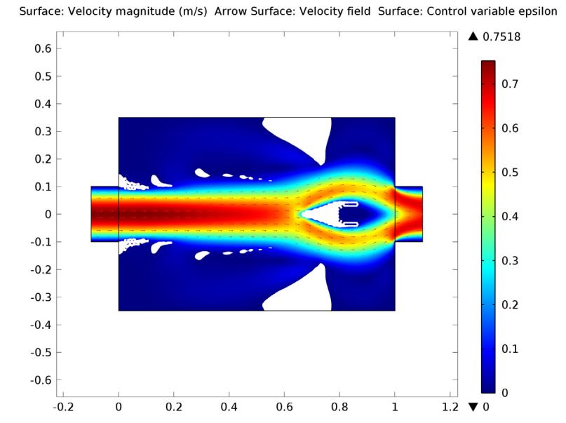
The magnitude of the fluid velocity.
Screenshot displaying the magnitude of the fluid velocity.

The app has three different solving options for computing just the flow field, computing just the separation using the existing flow field, or combining the two. A warning message is shown if there is not a clean separation.

Increasing the applied voltage will increase the magnitude of the DEP force. If the separation efficiency isn’t high enough, we can increase the voltage and click on the Compute All button, since in this case, both the fields and particle trajectories need to be recomputed. We can control the value of the Clausius-Mossotti function of the DEP force expression by changing the frequency. It turns out that at the specified frequency of 100 kHz, only red blood cells will exit the lower outlet.

The fluid permittivity is in this case higher than that of the particles and both the platelets and the red blood cells experience a negative DEP force, but with different magnitude. To get a successful overall design, we need to balance the DEP forces relative to the forces from fluid drag and Brownian motion. The figure below shows a simulation with input parameters that result in a 100% success in separating out the red blood cells through the lower outlet.

A screenshot shows the successful separation of red blood cells.
Successful separation of red blood cells.

Further Reading

To learn more about dielectrophoresis and its applications, click on one of the links listed below. Included in the list is a link to a video on the Application Builder, which also shows you how to deploy applications with COMSOL Server™.

Windows is either a registered trademark or trademark of Microsoft Corporation in the United States and/or other countries.

Which Multiphase Flow Interface Should I Use?

$
0
0

If you are interested in using COMSOL Multiphysics software to solve multiphase flow problems, you may be wondering which multiphase flow interface to choose. This is your guide to the six interface options available to you and when you should use them.

Overview of Applications and Multiphase Flow Interfaces

The COMSOL Multiphysics software’s multiphase flow capabilities cover a wide range of applications, including:

  • Bubbly flow
    • Discrete gaseous bubbles in a continuous liquid
  • Droplet flow
    • Discrete fluid droplets in another fluid
  • Particle-laden flow
    • Discrete solid particles in a fluid
  • Free-surface flow
    • Immiscible fluids separated by a clearly defined interface
  • Fluidized beds
    • Vertical cylinder containing particles where gas is introduced through a distributor

These application areas are covered by six different physics interfaces, and it is not always trivial to determine which physics interface is better suited to solve your particular application.

The six interfaces in the model tree.
Screenshot of the model tree displaying the six interfaces.

In this blog post, we describe these six multiphase flow physics interfaces to make it easier for you to choose. Very specific application areas, such as two-phase flow in porous media or cavitation problems, will be the object of future blog entries.

Interface Tracking vs. Disperse Methods

The six multiphase flow models can be split into two main categories, which we will refer to as the interface tracking methods and the disperse methods.

The interface tracking methods model the flow of two different immiscible fluids separated by a clearly defined interface. These methods are typically used to model bubble or droplet formation, sloshing tanks, or separated oil/water/gas flow. In the below example by the Philips® FluidFocus team, the meniscus between two immiscible liquids is used as an optical lens.

A meniscus between two immiscible liquids is used as an optical lens.
Image credit: Philips.

The shape of the meniscus in this device is controlled by changing the voltage applied to the conducting liquid, thus changing the focal point of the lens. The lens is then integrated within a miniature variable-focus camera. Because the exact location of the interface is of interest here, the FluidFocus team used an interface tracking method in their numerical model.

A tutorial showing how to reproduce this model can be found in our Model Gallery.

While the interface tracking methods are accurate and provide a clear picture of the flow field (velocity, pressure, and surface tension force), they are not always practical due to their high computational cost. Thus, the interface tracking methods are generally better suited to microfluidics problems in which only a few droplets or a few bubbles are tracked.

Larger-scale simulations involving a greater number of bubbles, droplets, or solid particles require computationally cheaper methods. Cue: the disperse methods.

This second category of methods does not explicitly track the position of the interface between the two fluids, but instead tracks the volume fraction of each phase, thus lowering the computational load. A circulated fluidized bed, which is a very common apparatus in the food, pharmaceutical, and chemical processing industries, can be modeled using a disperse method.

In this example, the dispersed phase, consisting of solid spherical particles, is fluidized by air and transported upwards through a vertical riser:

A model showing the dispersed phase traveling upward through a vertical riser.

Tracking every single solid particle would not be computationally practical here. Instead, we compute the volume fraction of solid particles. The disperse methods are typically used to model particle-laden flow, bubbly flow, and mixtures.

In the next few sections of this blog post, I will discuss and compare the different tracking and homogeneous methods.

Disperse Methods

The disperse methods include the following:

  1. Euler-Euler model
  2. Bubbly flow model
  3. Mixture model

Euler-Euler Model

The Euler-Euler model simulates the flow of two continuous and fully interpenetrating incompressible phases. Typical applications are fluidized beds (solid particles in gas), sedimentation (solid particles in liquid), or transport of liquid droplets or bubbles in a liquid.

This model requires the resolution of two sets of Navier-Stokes equations, one for each phase, in order to calculate the velocity field for each phase. The volume fraction of the dispersed phase is tracked with an additional transport equation.

The Euler-Euler model is the correct two-phase flow method to model the fluidized bed that I presented earlier. The model relies on the assumption that the dispersed particles, bubbles, or droplets are much smaller than the grid size.

The Euler-Euler model is the most versatile of the three disperse models, but it comes at a high computational cost. The model solves for two sets of the Navier-Stokes equations, instead of one, which is the case for all other models presented here. Both the bubbly flow and mixture models are simplifications of the Euler-Euler model and rely on additional assumptions.

Bubbly Flow Model

The bubbly flow model is used to predict the flow of liquids with dispersed bubbles. It relies on the following assumptions:

  • The dispersed bubbles are much smaller than the grid size
  • The gas density is negligible compared to the liquid density
  • The gas volume fraction does not exceed 10%

In this model of an airlift loop reactor, air bubbles are injected at the bottom of a reactor filled with water:

An image depicting an airlift loop reactor.

The bubbly model solves one set of Navier-Stokes equations for the flow momentum, a mixture-averaged continuity equation, and a transport equation for the gas phase. Although this model does not track individual bubbles, the distribution of the number density (i.e., the number of bubbles per unit volume) can still be recovered. This can be useful when simulating chemical reactions in the mixture.

Mixture Model

The mixture model is used to simulate liquids or gases containing a dispersed phase. The dispersed phase can be bubbles, liquid droplets, or solid particles, which are assumed to always travel with their terminal velocity. While this model can be used for bubbles, it is recommended to use the bubbly flow model instead for gas bubbles in a liquid.

The mixture model solves one set of Navier-Stokes equations for the momentum of the mixture, a mixture-averaged continuity equation, and a transport equation for the volume fraction of the dispersed phase. Like the bubbly model, the mixture model can also recover the number of bubbles, droplets, or dispersed particles per unit volume.

The mixture model relies on the following assumptions:

  • The density of each phase is constant
  • The dispersed phase droplets or particles travel with their terminal velocity

This tutorial models the flow of a dense suspension consisting of light, solid particles in a liquid placed between two concentric cylinders.

A model illustrating particle concentration.
Particle concentration.

Summary of the Disperse Models

I have summarized the disperse models for you in a table:

Euler-Euler Model Bubbly Flow Model Mixture Model
Valid for these continuous phases:
  • Liquid
  • Gas
  • Liquid
  • Liquid
Valid for these dispersed phases:
  • Particles
  • Bubbles
  • Droplets
  • Bubbles
  • Particles
  • Bubbles (the bubbly flow model is preferred for gas bubbles in a liquid)
  • Droplets
Assumptions:
  • The dispersed particles, bubbles, or droplets are much smaller than the grid size
  • The density of each phase is constant
  • The dispersed bubbles are much smaller than the grid size
  • The gas density is negligible compared to the liquid density
  • The gas volume fraction does not exceed 10%
  • The dispersed particles or droplets are much smaller than the grid size
  • The density of each phase is constant
  • The dispersed phase droplets or particles travel with their terminal velocity
Equations solved for (laminar flow):
  • 2 sets of Navier-Stokes equations
  • 1 continuity equation
  • 1 transport equation
  • 1 set of Navier-Stokes equations
  • 1 continuity equation
  • 1 transport equation
  • 1 set of Navier-Stokes equations
  • 1 continuity equation
  • 1 transport equation
Available turbulence models:
  • RANS, k-ε
  • RANS, k-ε
  • RANS, k-ε

These three multiphase flow models require the CFD Module. The mixture model for rotating machinery problems also requires the Mixer Module. More details on the required COMSOL products can be found in our specification chart.

Interface Tracking Methods

The interface tracking methods include:

  1. Level set method
  2. Phase field method
  3. Two-phase flow moving mesh method

All these methods very accurately track the position of the interface between the two immiscible fluids. They account for differences in density and viscosity of the two fluids, as well as effects of surface tension and gravity.

The Level Set and the Phase Field Methods

With the level set and phase field methods, the interface is tracked using an auxiliary function, or color function, on a fixed mesh.

The Navier-Stokes equations and the continuity equation are solved for the conservation of momentum and mass, respectively. The color function, and therefore the interface position, is tracked by solving additional transport equations (one additional equation for the level set method and two additional transport equations for the phase field method). This color function varies between a low value (0 and -1 for the level set and phase field methods, respectively) in one phase and high value of 1 in the second phase.

The interface is diffuse and centered on the center value of these functions (0.5 and 0 for the level set and phase field methods, respectively). The material properties of both phases such as the density and viscosity are scaled according to the color function.

A plot showing the filling of a capillary channel.

This plot shows the filling of a capillary channel using the level set or phase field method. The higher value of the color function (red region) shows the location of the fluid phase, while the lower value (blue region) represents the gas phase. The two phases are separated by a diffuse interface that is not aligned with the fixed mesh.

The phase field method, which is physically motivated, is generally more numerically stable than the level set method and is compatible with fluid-structure interactions. The level set method, however, usually represents surface tension slightly more accurately than the phase field method.

Moving Mesh Method

Unlike the level set and phase field methods, which are solved on a fixed mesh, the two-phase flow moving mesh method tracks the interface position with a moving mesh using the ALE method.

The moving mesh method.

Here, the same capillary filling simulation is implemented using the moving mesh method. This time, the interface is sharp and it follows the boundary between the fluid and the gas domain. Because the position of the interface is given by the boundary between the two meshes, it does not require any additional transport equations. Only one set of Navier-Stokes equations is solved on each mesh.

Since physical interfaces are usually much thinner than practical mesh resolutions, the two-phase flow moving mesh technique offers the most accurate representation of the interface. This method also accounts for mass transport across the interface, which is very difficult to implement using the two other interface tracking methods. Finally, the sharp interface also means that different physics can be solved in the domains on either side of the interface.

The main drawback of the moving mesh methods is the fact that the mesh must deform continuously, which means that problems involving topological changes cannot be solved. This drastically limits its applications. Problems such as droplet breakup or the transition from jetting to dripping of a liquid jet cannot be modeled using the moving mesh method and require the level set or phase field method. This jet instability simulation shows the break-up of a jet into droplets over time using the level set method.

A jet instability simulation.
Liquid regions (shown in black).

Tutorials for the droplet breakup and jet instability simulations are available in the Model Library and our online Model Gallery.

Comparison of the Interface Tracking Methods

As with the homogeneous models above, I have put the interfacing tracking methods in a table for an easy overview:

Level Set Phase Field Moving Mesh
Applicability: A check. A check. An error.
Does not support topological changes
Accurate representation of the interface: Better Good Best
Speed and convergence: Good Better Best
Equations solved for:
  • 1 set of Navier-Stokes equations
  • 1 continuity equation
  • 1 transport equation
  • 1 set of Navier-Stokes equations
  • 1 continuity equation
  • 2 transport equations
  • 1 set of Navier-Stokes equations
  • 1 continuity equation
  • No transport equations
  • ALE moving mesh
Available turbulence models:
  • RANS, k-ε
  • RANS, k-ε
  • None
Required COMSOL products for laminar flow:
Required COMSOL products for turbulent flow:

Conclusion

In this blog post, we compared six different two-phase flow methods. The COMSOL Multiphysics simulation software does offer additional multiphase flow methods, including two-phase flow methods in porous media or cavitation in thin films, such as journal bearings. These topics will be the object of future blog entries.

If you have any multiphase flow modeling questions, feel free to contact our Technical Support team. If you are not yet a COMSOL Multiphysics user and would like to learn more about our software, please contact us via this form — we’d love to connect with you.

PHILIPS is a registered trademark of Koninklijke Philips N.V.


Tears of Wine and the Marangoni Effect

$
0
0

Try pouring some wine into a glass. Don’t drink it yet — this is a scientific experiment. When you hold up your glass, you’ll see what look like teardrops running down the sides. These tears of wine are caused by the Marangoni effect, which describes a mass transfer along the surface of two fluid phases caused by surface tension gradients along the interface between the two phases (for example liquid and vapor).

Tears of Wine

The term tears of wine was first coined in 1865 by physicist James Thomson, the brother of Lord Kelvin. Italian physicist Carlo Marangoni later studied the topic for his doctoral research and published his findings in 1865. The Marangoni effect, which causes tears of wine and other phenomena observed in surface chemistry and fluid flow, is named after Marangoni and his research.

A glass with tears of wine caused by the Marangoni effect.
Tears of wine moving down the inside of the glass.

The Marangoni Effect in Action

Study your glass. Do you see the tears? If not, it may be because you chose a wine of low alcohol content. If you want to see tears of wine, wine with a high alcohol content is more likely to display tears. Wine with a low alcohol content gives only small variations in alcohol concentration and surface tension along the wine-air interface and will rarely show teardrops. The wine in the photo above has 13.5% alcohol content, which is on the lower side, but high enough to produce tears.

Surface tension is a property of the interface between two phases. It describes the amount of energy needed to expand the surface area of that interface by one unit. You can also look at surface tension as the force per unit length needed to create new surface area. The figure below illustrates a liquid phase in contact with its vapor. The surface molecules (shown in red) have only very small upwards interactions with the vapor molecules (shown in orange) causing them to experience asymmetrical force that pulls the surface of the liquid together. The molecules in the bulk of the liquid (blue) interact in all directions. To expand the surface area of the liquid, bulk molecules have to move towards the surface, breaking up upward interactions. Doing so requires energy.

A diagram depicting surface tension in a liquid that is interacting with its vapor.
Surface tension in a liquid interacting with its vapor. The molecules at the surface (red) experience asymmetric interactions. The molecules just below (violet) experience slightly more symmetric interactions, while the molecules in the bulk (blue) experience even more symmetric interactions.

Water has strong interactions in the bulk of the liquid due to its hydrogen bonds, so it has a relatively large surface tension since it requires breaking strong interactions. Liquids-vapor interfaces have surface tensions that depend on the strength of the interactions between the molecules in the bulk of the liquid. The Marangoni effect is the flow caused by gradients in surface tension along the liquid-vapor interface surface in the figure above. Such a gradient can be caused by differences in composition or temperature of the solution along this surface.

We can see how this works by pouring a thin layer of water onto a plate and adding glitter or another kind of light material to better illustrate the effect. The interaction between the water and the glitter is due to the glitter particles being hydrophilic, or water loving. Adding a drop of soapy solution, alcohol, motor oil, or any liquid with a contrasting surface tension to the center of the surface causes all of the glitter to immediately rush to the sides of the surface, away from the center.

As you pour soap, the soap molecules form a thin film — only one or a few molecules thick — on the water surface. The surface experiences a difference in surface tension between the parts covered by soap and the parts with only water, which causes the soap film to spread and the glitter particles to flow to the sides — the Marangoni effect. Eventually, the soap molecules cover the whole surface, which lowers the surface energy, because now the surface water molecules are also able to interact with the hydrophilic end of the soap molecules.

In the next figure, the experiment is illustrated on a molecular level. The glitter particles rather interact with water, not with soap, because they have a hydrophilic surface. They are squeezed to the sides as the soap covers the surface because they “want” to continue interacting with water molecules.

An illustration of how surface tension changes when soap is added to water.
Surface tension changes as soap is added to water. Soap is green, an ion with with a hydrocarbon “tail”. Water is blue in the bulk, red at the free water surface, and violet at the surface covered by soap or when they are just below other surface water molecules.

Three plates with water, glitter, and soap to demonstrate the Marangoni effect.

In tears of wine, a meniscus forms at the three-phase junction between the wine glass walls, wine, and air. This is where the liquid loosely clings to the surface of the glass. The meniscus is formed because the walls of the glass have a hydrophilic surface, like the surface of the glitter particles. Wine contains alcohol that is continuously evaporating from the surface at a rate higher than water (since ethanol has a higher equilibrium vapor pressure than water), and this also takes place in the meniscus. The alcohol concentration decreases faster in the meniscus due to its higher surface area in relation to its small volume. Therefore, it causes an alcohol concentration difference between the meniscus and the flat interface surface between the wine and air. This then causes a surface tension gradient that moves the meniscus up the walls of the glass.

As the meniscus begins to form a film on the surface of the glass’ walls, it gets even more depleted of alcohol, which in turn causes a larger surface tension gradient. More wine gets pulled up the walls of the glass until droplets form. Gravity takes effect and tears of wine run down the sides of the glass and back into the bulk of the wine.

A diagram explaining how tears of wine form.
Tears of wine form due to the surface tension (γ) gradient between the meniscus and the flat surface of the wine.

Here’s a 3-second time-lapse video to further illustrate the effect:


Modeling the Marangoni Effect, a Jet Instability Model

We can model the Marangoni effect with COMSOL Multiphysics and the Microfluidics Module. To get started, we have a tutorial model that illustrates the concept — the Jet Instability model. This model simulates an inkjet printer and the break-up of an infinitely long liquid jet due to a spatially varying surface tension coefficient.

There are three ways to solve this model: via the moving mesh, level set, or phase field methods. If you go to the Model Gallery, you will find PDFs with modeling instructions for two of these (the moving mesh and level set methods). The moving mesh method is faster and easier to use than the level set method, as we saw in Fabrice Schlegel’s blog post Which Multiphase Flow Interface Should I Use? However, we can only use the moving mesh method to model the Marangoni effect in tears of wine if the wine layer on the side of the glass has a definite thickness. There can be no dry area between the tears and the rest of the wine. If that’s the case, we must use either the level set or the phase field method.

The Jet Instability model consists of a fluid domain in the shape of a cylinder with a radius of 20 microns and a height of 60 microns. The domain contains a cylinder of water with a radius of 5 microns. We need to define the ink properties such as density and dynamic viscosity, as well as the surface tension coefficient.

We use the Laminar Two-Phase Flow, Moving Mesh interface to solve the model, which is plotted on moving mesh geometry. For this simulation, the interface has no thickness and is represented by a boundary. This is better for practical mesh densities. The interface calculates the Navier-Stokes equations and boundary conditions and transforms it onto a fixed mesh.

A surface plot of a cylinder of an inkjet printer created with COMSOL Multiphysics.
A cylinder of an inkjet printer in the Jet Instability model.

The Laminar Two-Phase Flow, Moving Mesh interface can easily input other physics and it is faster and more accurate than the level set and phase field methods. However, the moving mesh method cannot handle topological changes. This means that it can only be used for calculations prior to the break-up of droplets. The Laminar Two-Phase Flow, Level Set interface calculates velocity field and pressure as described by the Navier-Stokes equations, periodic boundary conditions, and point settings.

The results below were modeled using the level set method and show the break-up of the jet into droplets over six time periods. At first, the liquid forms a perfect column, but the variation in surface tension disturbs the jet and causes a force due to surface curvature that eventually breaks up the jet into droplets.

A jet instability model made with the level set method.
The liquid regions of the model as the jet breaks up due to surface tension variation over time.

Further Reading

Ps. We’re currently working on a new Heat Transfer feature for modeling Marangoni convection. Stay tuned for the upcoming release of COMSOL Multiphysics version 5.1…

Simulating Analog-to-Digital Microdroplet Dispensers for LOCs

$
0
0

Microfluidic biochips have a variety of applications and are valued for their low cost, fast response time, and high efficiency. In the paper “Design and Simulation of High-Throughput Microfluidic Droplet Dispenser for Lab-on-a-Chip Applications”, which was presented at the COMSOL Conference 2014 Boston, researchers designed a microfluidic biochip with an analog-to-digital converter. They used COMSOL Multiphysics software to understand the mechanism of the device and verify its function.

Microfluidic Biochips and the Need for Analog-to-Digital Converters

In the field of MEMS and lab-on-a-chip devices, microfluidic biochips don’t require a lot of power or sample volume to operate. They are also relatively cheap, offer a fast response time, and are overall highly efficient. Another great advantage is their ability to integrate operations such as detection, sample pre-treatment, and sample preparation onto a single chip. Microfluidic biochips are used in a wide range of applications, including inkjet printer heads, micro drug delivery systems, and DNA and clinical pathology devices.

There are two kinds of microfluidic biochips:

  1. Analog, which handle continuous flow.
  2. Digital (DMFBs), which rely on electrowetting-on-dielectric (EWOD) techniques to drive droplets to move, merge, split, or be manipulated to perform other functions.

Generally, microfluidic samples are continuous flow, such as drops of blood or saliva for diagnostic tests. This leads to two problems: You cannot control the droplet volume and the excess liquid can’t be removed in the case of overpressure on the device. In cases like these, for analog microfluids to be processed by a DMFB, an analog-to-digital converter (ADC) is needed on the device.

ADCs are microfluidic dispensers that can dispense manipulated droplets from continuous flow or a reservoir of the sample. These devices are fundamental for integrating analog and digital microfluidic biochips into a mixed-signal microfluidic device. Surprisingly, there is not a great amount of research on integrating an ACD into a microfluidic biochip design. Answering the call, a team of researchers from the University of Bridgeport in Connecticut set out to design and simulate a high-throughput microfluidic droplet dispenser as an analog-to-digital microfluidic converter for use in lab-on-a-chip (LOC) applications.

A diagram showing a microfluidic droplet dispenser.
A schematic of a microfluidic droplet dispenser. Image credit: C. Jin, X. Xiong, P. Patra, R. Zhu, J. Hu, University of Bridgeport, Bridgeport, Connecticut. Taken from their COMSOL Conference 2014 Boston paper submission.

Designing and Simulating an Efficient Device

The research team aimed to understand the mechanism of a high-throughput droplet dispenser as well as verify its function as an interface between analog and digital microfluidic biochips on an LOC device.

First, they used the Laminar, Two-Phase Flow interface with the level set method in COMSOL Multiphysics to simulate the droplets as they move and split in the dispenser by simulating the electrowetting process. This was done to better understand microfluidic behavior in general and analyze the time settings needed for the next phase of the simulation. The researchers were also able to calculate the force needed to move the droplets, evaluate the droplet shape and movement, as well as analyze the voltage needed to cause their movement.

This schematic shows moving microfluidic droplets located in a dispenser.
Simulating microfluidic droplets in a dispenser as they move and split. Image credit: C. Jin, X. Xiong, P. Patra, R. Zhu, J. Hu, University of Bridgeport, Bridgeport, Connecticut. Taken from their COMSOL Conference 2014 Boston paper submission.

Next, the team simulated the droplet dispenser as an interface between analog and digital microfluidic flow. To reduce simulation time, only two digital output ports were included on the model. With COMSOL Multiphysics, the team easily selected mesh elements to create a finer meshed model of the droplet dispenser.

Here, the digital droplet dispenser is displayed as a meshed model.
A meshed model of the digital droplet dispenser. Image credit: C. Jin, X. Xiong, P. Patra, R. Zhu, J. Hu, University of Bridgeport, Bridgeport, Connecticut. Taken from their COMSOL Conference 2014 Boston paper submission.

The behavior of the droplets in the output ports was simulated in both alternate and parallel modes to analyze the efficiency of each method.

This image shows the droplet dispenser in parallel mode.
An image depicting the droplet dispenser in alternate mode.

Simulating the parallel (left) and alternate (right) modes of a droplet dispenser allows researchers to analyze the behavior of the device. Image credit: C. Jin, X. Xiong, P. Patra, R. Zhu, J. Hu, University of Bridgeport, Bridgeport, Connecticut. Taken from their COMSOL Conference 2014 Boston paper submission.

After simulating the droplet dispenser, the researchers verified its function and further concluded that dispensing the droplets in both alternate and parallel modes works effectively for integrating analog and digital microfluidics on a single lab-on-a-chip device. Hopefully, this research will inspire more improvements to these devices, advance the field of microfluidics, and in turn improve clinical diagnostics and other applications.

Further Reading

To learn more about the digital droplet dispenser, download the paper and presentation from the COMSOL Conference 2014 Boston: “Design and Simulation of High-Throughput Microfluidic Droplet Dispenser for Lab-on-a-Chip Applications“.

Simulating a Valveless Micropump Mechanism

$
0
0

Microfluidic systems often rely on valveless pumps, as they are both gentle on the biological material and low in the risk of clogging. However, by design, this type of pump is not suitable for viscous fluids and systems with small length scales or low flow rates. To overcome this limitation, you can introduce a micropump mechanism that converts oscillatory fluid motion into a unidirectional net flow.

What Is a Valveless Micropump?

Miniature devices have many applications and researchers are constantly finding new uses for them. One such use, which we’ve blogged about before, is a microfluidic device that could let patients conduct immune detection tests by themselves. But to work in the microscale, devices like this one, of course, rely on even smaller components such as micropumps.

Let’s turn to a tutorial model of a valveless micropump mechanism that was created by Veryst Engineering, LLC using COMSOL Multiphysics version 5.1.

The micropump in the tutorial model creates an oscillatory fluid flow by repeating an upstroke and downstroke motion. The fluid flow enters a horizontal channel containing two tilted microflaps, which are located on either side of the micropump. The microflaps passively bend in reaction to the motion of the fluid and help to generate a net flow that moves in one direction. Through this process, the micropump mechanism is able to create fluid flow without the need for valves.

The geometry of a micropump.
The geometry of the micropump mechanism tutorial.

Please note that the straight lines above the microflaps are there to help the meshing algorithm. Check out the tutorial model document if you’d like to learn how this model was created.

Evaluating the Micropump’s Performance with Simulation

The tutorial calculates the micropump mechanism’s net flow rate over a time period of two seconds — the amount of time it takes for two full pumping cycles. The Reynolds number is set to 16 for this simulation so that we can evaluate the valveless micropump mechanism’s performance at low Reynolds numbers. The Fluid-Structure Interaction interface in COMSOL Multiphysics is instrumental in taking into account the flaps’ effects on the overall flow, as well as making it an easy model to set up.

The mechanism in a pumping downstroke.
The mechanism in a pumping upstroke.

Left: At a time of 0.26 seconds, the fluid is pushed down and most of it flows to the outlet on the right. Right: At a time of 0.76 seconds, the fluid is pulled up and most of it flows from the inlet on the left.

The simulation starts with the micropump’s downstroke, which is when the micropump pushes fluid down into the horizontal channel. This action causes the microflap on the right to bend down and the microflap on the left to curve up. In this position, the left-side microflap is obstructing the flow to the left and the flow channel on the right is widened. This naturally causes the majority of the fluid to flow to the right, since it is the path of least resistance.

During the following pumping upstroke, fluid is pumped up into the vertical chamber. Here, the flow causes the microflaps to bend in opposite directions from the previous case. This shift doesn’t change the direction of the net flow, because now the majority of the fluid is drawn into the flow channel from the inlet on the left.

Due to the natural deformation of the microflaps caused by the moving fluid, both of these stages created a left-to-right net flow rate. But how well did the micropump mechanism do at maintaining this flow over the entire simulation time period?

A plot of the net volume pumped left to right.
The net fluid volume that is pumped from left to right.

During the two-second test, the net volume pumped from left to right was continually increased, with a higher net flow rate during peaks of the stroke speed. This valveless micropump mechanism can function even at a lower Reynolds number.

The valveless micropump mechanism could have many future applications, one of which is to work as a fluid delivery system. In such a scenario, a micropump mechanism could take fluid from a droplet reservoir on its left and move it through a microfluidic channel to an outlet on its right. In this post we have shown just one set of simulation results. By experimenting with the tutorial model set up by Veryst Engineering, you can visualize how a valveless micropump may work in different situations and use this information to discover new uses for micropump mechanisms.

Try It Yourself

Creating Ultrafast Polymerase Chain Reaction Tests with LEDs

$
0
0

Polymerase chain reaction tests have many applications within medical and biological research. In the past, these tests have been performed within a laboratory setting due to their high power requirements and the slow speed at which results are delivered. Researchers at the University of California, Berkeley have developed a new LED-based polymerase chain reaction system that, with its simplicity and speed, could be used in point-of-care testing.

Point-of-Care Testing: Combining Convenience with Faster Results

Laboratory test results provide clinicians with important insight into the best treatment methods for their patients. However, there is often a period of waiting between the time of testing and when the results are made available — a time frame that can range from several hours to even days. With this waiting period comes delays in starting patients’ treatments, as the clinicians must obtain the test results before they can move forward in their assessments.

In recent years, there has been a healthcare industry shift from such conventional laboratory tests to rapid point-of-care testing. Point-of-care testing refers to simple medical tests that deliver fast results and can be conveniently performed in a variety of settings, from the home to a physician’s office. Along with increasing patients’ roles in managing their healthcare, these tests expedite clinicians’ decision-making processes, allowing them to suggest treatments more quickly. As noted in a 2010 report from the National Institutes of Health, accelerating this process can greatly enhance the delivery of healthcare as well as address issues relating to health disparities.

Blood glucose test strips are one example of point-of-care testing.
A simple method for testing blood glucose. Image by Karl101 — Own work, via Wikimedia Commons.

So what types of point-of-care tests are available today? Blood glucose testing, pregnancy testing, food pathogen screening, and cholesterol screening are some common examples. As technologies continue to grow, point-of-care testing is becoming a viable option for more and more laboratory-based clinical tests. Such is the case for polymerase chain reaction (PCR) tests.

The Development of Polymerase Chain Reaction Tests

Polymerase chain reaction is a technology that is designed to copy small segments of DNA with the goal of generating enough sequences to perform analyses. This method of DNA amplification relies on thermal cycling. As the particular DNA segment of interest is exposed to repeated cycles of heating and cooling, the molecule is amplified at an exponential rate.

The roots of PCR technology can be traced back to the work of H. Gobind Khorana and Kjell Kleppe in 1966. Through a process they deemed repair replication, a small synthetic DNA molecule was duplicated and then quadrupled via two primers (short nucleic acid sequences) and DNA polymerase (enzymes that create DNA molecules by assembling nucleotides).

Using this initial research as his foundation, Kary Mullis, an American biochemist, added repeated thermal cycling into the mix. Through this cycling process, DNA sequences could be rapidly copied, with the amplification becoming increasingly fast over time. Several years later, a thermostable DNA polymerase — Taq polymerase — was implemented within the process. This DNA polymerase automated the thermocycler-based process, removing the need for continuous handling throughout amplification.

Polymerase chain reaction test tubes.
Adding PCR tubes to a thermal cycler.
Top: PCR test tubes. Image by Madprime — Own work, via Wikimedia Commons. Bottom: Adding PCR test tubes to a thermal cycler. Image by Karl Mumm — Own work, via Wikimedia Commons.

The polymerase chain reaction process can be broken down into a series of steps:

  1. The select DNA molecule is exposed to heat to separate the double-stranded DNA molecule into single strands — a process known as denaturation. DNA must be separated into single strands in order to be copied.
  2. The reaction temperature is reduced so that the primers can anneal to their matching sequences on the initial DNA strand. The DNA polymerase then binds to the annealed primer.
  3. The DNA polymerase synthesizes a new strand of DNA, using the single-stranded DNA molecule and the primers as a template. The amplification process continues exponentially.

PCR tests have found use in a variety of medical and biological applications, including DNA cloning, the identification of genetic fingerprints, and the detection and diagnosis of infectious diseases. These tests typically take an hour or so to complete and utilize a conventional heater that is both expensive and requires a lot of power. As such, PCR tests have not been practical for point-of-care testing in the past. A recent design, however, could lead to new advancements.

LED-Based Design Extends the Use of PCR Tests

Looking to advance the speed of conventional PCR tests, a team of researchers at UC Berkeley turned to the power of LEDs. In their experiments, the researchers used thin films of gold deposited onto a plastic chip featuring microfluidic wells. These wells, which the LEDs were positioned underneath, were designed to hold the PCR mixture with the sample of DNA. As part of their research, the team performed electromagnetic simulations using COMSOL Multiphysics to help define their geometry and material parameters.

With the LEDs in place, the electrons at the interface of the gold films and a DNA solution were successfully heated. Such behavior can be explained by plasmonics, which describes the interaction between light and free electrons on the surface of a metal. When exposed to light, free electrons become excited and begin to oscillate, causing heat to be generated. When the lights turn off, the oscillations stop and heat is no longer produced.

The research team found that their plasmonic PCR system helped to speed up the thermal cycling process, generating test results within a matter of minutes. Comparing their design with conventional PCR tests, the researchers found that both methods compared well in their ability to amplify a sample of DNA. With its simple, low-cost design and ability to deliver fast results, this LED-based system could help bring PCR tests outside of the laboratory and into a variety of environments.

Further Reading

Focusing on an Electrowetting Lens

$
0
0

Adjusting the focal length of a camera lens allows you to change your angle of view. Miniature lenses can achieve this change by using a method called electrowetting. Electrowetting involves changing the balance of forces at a contact point of a free surface and a solid by applying a voltage. However, focus is not obtained immediately due to oscillations in the free surface. Here, we investigate the optimal viscosity for critically damping the free surface when a voltage is applied.

A Quick Introduction to Focal Length

Imagine that you’re taking a photo and zooming in and out to see what looks best. In this moment, you are using a variable-focus lens to change the focal length of your camera. Focal length is the distance between the optical center or point of convergence of your lens and your camera’s sensor when a subject is in focus.

A shorter focal length yields a wider angle of view and thus a zoomed out view of your subject. A longer focal length provides a zoomed in and narrow angle of view.

Picture example of a shorter focal length.
Photograph showing a longer focal length.

Left: A shorter focal length. Right: A longer focal length.

In order to adjust their focal length, traditional variable-focus lenses use moving parts that may not function on a miniature scale. Instead, miniature lenses can use alternative processes such as electrowetting to change their focal length.

Developing a Miniature Fluid Lens Using Electrowetting

Electrowetting is the process of applying a voltage between a conducting fluid and a solid surface in order to modify the balance of forces at the contact point. In the case of a lens, this can change the meniscus shape of a liquid and so alter the focal length of the lens.

For example, let’s look at a tutorial model based on an electrowetting lens developed by the Philips FluidFocus team.

This tutorial model consists of a sealed chamber with two immiscible liquids: a lower conducting fluid and an upper insulating fluid. Both fluids have a matching density and viscosity. The tutorial also utilizes a technique called electrowetting on dielectric (EWOD), which involves using a thin dielectric deposited onto a conducting layer as the solid surface.

When the voltage applied to the conducting liquid of the lens is increased, the meniscus curvature changes from convex to concave, as pictured below.

A diagram showing the workings of the Philips FluidFocus lens.
A change in curvature due to electrowetting. When a voltage is applied, the curvature changes from A to B. Image credit: Philips.

This change occurs because the wetting properties of the surface are altered by the voltage, causing the fluid to change position in response. The modified curvature changes the focal length, which allows us to use the meniscus between these two liquids as a variable-focus optical lens.

Although the design we’ve described so far is functional, it may not allow you to quickly change focal lengths. This is an issue because you don’t want to wait for your camera lens to adjust positions every time you need to change the focal length. To avoid this, we can optimize the electrowetting process to create a lens with the fastest possible response time.

Optimizing an Electrowetting Lens with Simulation

As we switch the voltage applied to the electrowetting lens, the contact angle of the fluid can change abruptly. We see this change happening in the following photos from Philips.

A photo showing how different applied voltages change the meniscus shape.
The change in meniscus shape for the following voltages: C: 0 V, D: 100 V , and E: 120 V. Image credit: Philips.

The movement creates a disturbance that produces capillary waves on the interface. This may result in oscillations that take time to decay. For instance, in this tutorial model, higher-order modes are still visible 2 ms after the voltage is switched from 100 V to 120 V.

A schematic illustrating the fluid velocity magnitude and direction in an electrowetting lens.
Image of the lens' fluid pressure fluid and velocity.

Images show the electrowetting lens 2 ms after the voltage changed from 100 V to 120 V. In both cases, the viscosity of the insulating fluid is 10 mPa·s. Left: Fluid velocity magnitude (color) and direction (arrows). Right: Pressure in fluid (color) and boundary velocity (arrows).

To optimize the lens, we want to facilitate quick focal length shifting by minimizing the oscillations of the meniscus that occur during this process. Therefore, the system needs to be critically damped to achieve the fastest possible response time.

In order to accomplish this, we can change the damping of the insulating fluid by adjusting its viscosity. This tutorial uses COMSOL Multiphysics® software Two-phase Flow, Moving Mesh interface to accurately model the flow of two different fluids and test different values of viscosity.

Plot comparing three viscosity values of the miniature fluid lens.
Comparing different values of viscosity by plotting the location of the center of the meniscus against time.

Of the tested viscosity values, it appears that 50 mPa·s is the closest to being critically damped, and is therefore the optimal viscosity for the insulating fluid of an electrowetting lens.

The Philips FluidFocus team used this interface tracking method in their own numerical model. With this, they were able to develop a miniature electrowetting lens that can change its focal length over a large range.

A photograph of the Philips miniature electrowetting lens and camera.
The PHILIPS® electrowetting lens and a camera that can contain the lens. Image credit: Philips.

You can test different viscosity values and analyze the physics of an electrowetting lens yourself by downloading the tutorial model.

Further Reading

PHILIPS is a registered trademark of Koninklijke Philips N.V

Simulate Three-Phase Flow with a New Phase Field Interface

$
0
0

In COMSOL Multiphysics version 5.2, the CFD and Microfluidics modules include a new fluid flow interface for modeling separated three-phase flow. The model behind this fluid flow interface accounts for surface tension between each pair of fluids, contact angles with the walls, as well as the density and viscosity of each of the fluids. The phase field method computes the shape of the interfaces between the three phases and also accounts for interactions with walls.

Modeling Separated Multiphase Flow

COMSOL Multiphysics has offered modeling and simulation capabilities for multiphase flow for many years. However, the equation-based formulation of three-phase flow problems has been used successfully by only a few experts in our user community, as seen in the figure below. In the last two or three years, we have received numerous requests for a more user-friendly, ready-made three-phase flow interface. In COMSOL Multiphysics version 5.2, we have satisfied these requests.

Results from a three-phase flow rotating drum simulation.
Simulation results of a rotating drum with three-phase flow, performed by a COMSOL Multiphysics user with equation-based modeling.

The description used in this new flow interface, the Three-Phase Flow, Phase Field interface, is a separated multiphase flow model. This interface is similar to the level set and phase field models for the two-phase flow interfaces included in earlier versions of the software. This means that the interface between the three immiscible phases (air, oil, and water, for example) is resolved in detail, including the effects of surface tension and contact angles.

Separated multiphase flow models are used for studying microfluidic systems and for fundamental studies of bubble coalescence and droplet breakup mechanisms. These are processes and phenomena where surface tension, contact angles, and buoyancy effects play a significant role on the shape of the phase boundaries between the different fluids and on the velocity field. Microfluidic devices and processes are typically found in analytical chemistry, biotechnology, medical technology, and nanotechnology. They include inkjets, sensors, separation devices, lab-on-a-chip devices, and microreactors.

High-fidelity separated multiphase flow models are usually too computationally expensive for direct use in macroscopic descriptions, since that may require resolving the surface of thousands or millions of droplets and bubbles. However, the results of detailed fundamental studies on a few bubbles and droplets can be used to develop simplified, less computationally expensive models. These simplified descriptions can usually be included in macroscopic dispersed multiphase flow models, which can describe systems with millions of bubbles and droplets. Macroscopic dispersed multiphase flow models are interesting in the study and design of devices and processes in the pharmaceutical, food, chemical, and household product industries.

The tutorial included in the Application Library, shown in the image below, deals with a droplet of air that rises through a layer of water at the bottom of a container and then into a layer of oil, lighter than water, resting on the water’s surface. As the air bubble moves through the water-oil interface, it carries some water in its wake and into the layer of oil. The water entrained in the bubble’s wake forms a “water tail” behind the bubble in the oil layer. This example is a benchmark from scientific literature, which we used to verify the equations in this fluid flow interface.

Images showing an air bubble penetrating a phase boundary separating water and oil.
An air bubble penetrates the phase boundary between water and oil and entrains a small amount of water in its wake. The entrained water droplet forms a tail behind the rising bubble.

This problem is interesting in a microfluidic system, since this mechanism can be used to transport small droplets of water into a layer of oil. The water droplets can, for example, be used to extract water soluble species from the oil into the water droplets, while keeping the hydrophobic species in the oil, to perform separation in a very controlled way. If the size of the water droplets is small enough, coalescence of the droplets in the oil phase may be avoided, thus creating droplets with a specific content and weight.

The same model can also be used to calculate the size distribution and coalescence kinetics, which can in turn be used in a dispersed multiphase flow model of an air-water-oil mixture. Emulsions can be used to create powders and structured mixtures.

The Physics and Model Behind the Three-Phase Flow, Phase Field Interface

The schematic below shows the three immiscible phases. The model is based on a free energy formulation of the system using three different phase field variables, with one for each phase (A, B, and C). The phase boundary is determined by the isosurface of a phase field variable for the value of 0.5, which corresponds to the pink and gray isosurfaces in the image above. The sum of all phase field variables in each point in space has to be equal to 1. The phase field variables are thus measures of the content of each phase in every point in space.

Illustration of a three-phase system.
A schematic drawing of the three-phase system, visualized in a projection plane perpendicular to the container walls.

The free energy equation is a function of the phase field variables and the surface tension for each pair of possible boundary interfaces, i.e., AB, AC, and BC. Each of the phase field functions is then used in the conservation equations for each field, which include the minimization of the free energy of the system. The formulated equations are the so-called Cahn-Hilliard equations.

Note also that this formulation accurately treats the triple point between the three phases, which is the point between the blue, pink, and white colored regions for phases A, B, and C shown above. This allows for the simulation of partial and absolute wetting between the three phases.

The interaction with the walls is determined by the contact angles in figure 2, θi, which are set to fixed values. The contact angles are used to express the boundary conditions for each of the phase field variables at the walls. Each angle is computed as the angle between an isosurface of the phase field variable at the value of 0.5, using the projection on a plane perpendicular to the walls, as shown above.

The surface tension forces in the system are also introduced in the equations for the conservation of momentum (Navier-Stokes equations) as sources of momentum. The density and viscosity, at each point in space in the equations for conservation of momentum and mass, are computed from the phase field variables, switching from the values of one fluid to another. Each phase gets the density and viscosity of the pure phase, which smoothly but rapidly changes across the phase boundary at the phase field value of 0.5.

The formulation described above is the one used in the phase field method, which is considered one of the most accurate ways of describing multiphase flow in continuum models.

An Intuitive User Interface

The user interface in the Three-Phase Flow, Phase Field interface in the CFD and Microfluidics modules is a so-called multiphysics interface. This means that, as a user, you have control of both the Cahn-Hilliard equations for the phase fields and the fluid flow equations. Although the settings are available in predefined formulations, an experienced user may also easily extend the equations to include other phenomena; for example, electric fields for studying electrocoalescence.

The image below shows the physics interfaces to the left, in the model tree, which are defined by the Three-Phase Flow, Phase Field interface. The included physics interfaces are the Laminar Flow and Ternary Phase Field interfaces. In addition, the Multiphysics node couples these two physics interfaces in its child node, the Three Phase Flow, Phase Field coupling node.

In the Ternary Phase Field interface, the Mixture node settings contain the input fields for surface tension, as shown below. In addition, the convection term is displayed, showing that the velocity field is obtained from the coupling formulated in the Three Phase Flow, Phase Field coupling node.

Screenshot showing the Mixture node.
The Mixture node contains the settings for the Cahn-Hilliard equations, which are the surface tension for the mixture and the coupling velocity field. The Equation section shows the domain equations.

The interaction with the container wall is defined by the settings for the Wetted Wall node, shown in the image below. Here, we find the input fields for the contact angles and a description of the notations used for these angles.

Screen capture showing the Wetted Wall boundary condition settings.
Settings for the Wetted Wall boundary condition, which sets the contact angles for the different phase boundaries with the walls of the container.

The settings for the Three Phase Flow, Phase Field coupling node are shown below. Here, we can see that the coupled physics interfaces are the Laminar Flow and Ternary Phase Field interfaces. For an advanced user, the coupling node gives the possibility to couple the Ternary Phase Field interface to different fluid flow interfaces, which may be defined in different ways or in different domains.

Image showing the Three Phase Flow, Phase Field coupling node settings.
The settings for the Three Phase Flow, Phase Field coupling node.

Possible Future Extensions to the Functionality

The first version of the Three-Phase Flow, Phase Field interface is formulated for laminar flow problems. A natural extension is to also formulate this model for turbulent flow. We are planning to offer this capability in a future release of COMSOL Multiphysics. Another natural addition is to include solid particles in the flow. This can, in fact, already be done using the Particle Tracing for Fluid Flow interface. We also plan to provide related Application Library examples in future software versions.

Further Reading

Model How the Bubbles in a Glass of Stout Beer Sink, Not Rise

$
0
0

When you think of a stout beer, one type that may come to mind is Guinness® beer. This stout is very special, noticeable by its dark body and famous white head. The dynamics of the foam alone are interesting enough to write a series of blog posts about. Although I don’t drink Guinness® beer (I’m a fan of IPA), I found the longstanding debate about whether its bubbles are rising or sinking while the beer settles makes an interesting simulation.

The Mystery of Sinking Bubbles in Stout Beer

Are the bubbles in a glass of Guinness® beer rising or sinking? An obvious reason why this question has never fully been answered is that most experimentation is carried out in pubs, and that might affect the judgment of researchers after five p.m. Recently, however, scientists have figured out the direction the bubbles move both experimentally (outside of bars!) and numerically using the COMSOL Multiphysics® software (see the Further Reading section). This blog post shows how to answer this question very quickly with a numerical method and provides a mechanistic understanding of the process.


Why would an application engineer who does not drink Guinness® beer be fascinated by the motion of its bubbles? It turns out that the dynamics between gas and bubbles have very important applications in many industries, such as the food, chemical, and biopharmaceutical industries. Bubble dynamics is also a very prevalent subject in academia.

Modeling Stout Bubbles in COMSOL Multiphysics

The Bubbly Flow interface is the appropriate choice for modeling bubble dynamics in stout beers. This interface, available in the CFD Module, solves for the beer’s velocity and pressure using the Navier-Stokes and mass conservation equations. It also solves for an additional transport equation to find out the concentration of bubbles in the beer. In other words, we are not individually tracking every single nitrogen bubble in the glass, as it would be too expensive from a computational point of view. Instead, we track the volume fraction of bubbles in the beer.

Material properties for the liquid phase and gas phase.
The material properties, i.e., the density and viscosity, for the liquid phase (beer) and gas phase (bubbles).

One specificity of stouts is the use of nitrogen rather than carbon dioxide during the carbonation process, leading to finer bubbles.

A screenshot depicting the physics interface setup.
The physics interface setup.

The geometry is built in the 2D axisymmetric mode in such a way that the total volume of the glass is equal to one pint. The side and bottom walls are set to the default No Slip velocity boundary condition with no gas flux through the glass.

Geometry of the glass.

The top boundary is set to a slip velocity and a gas outlet, thus mimicking the free surface between the beer and the foam. The foam is not modeled here.

Boundary selections for the model.

A fully structured (mapped) mesh is built with boundary layer elements near the walls to fully resolve the high velocity gradient in the neighborhood of these walls. Note that the default physics-based triangular mesh with boundary layer elements can be used as well. More information on meshing can be found in quite a few previous blog posts.

A fully mapped mesh for the glass.
Fully mapped mesh for the glass.

Are the Bubbles Rising or Sinking?

You naturally expect bubbles to float to a surface through buoyancy. Yet in any Irish pub, you can verify that with proper glasses, the bubbles sink. So, what is going on? To answer, we run our simulation for two minutes. The results after 1.5 seconds are shown below:

A simulation showing the volume fraction of bubbles after 1.5 seconds.
Volume fraction of bubbles after 1.5 seconds.

The color contour plot above shows the volume fraction of bubbles. The initial volume fraction of bubbles is 2%. After 1.5 seconds, this value is lower at the bottom of the glass and near the side wall. Earlier, I mentioned “Irish pubs with proper glasses” because the shape of the glass is very important in creating this effect. The bubbles have been observed to sink for glasses that widen toward the top and rise for glasses that widen toward the bottom.

A schematic showing the rising of bubbles.
As seen in this schematic, rising bubbles in a glass with a wider top create a thin layer close to the wall with a lower density of bubbles immediately after the beer has been poured. Therefore, the liquid-gas mixture has a higher density close to the wall.

A second or two after being poured, the fluid is close to being at rest. Because of buoyancy, the lower density fluid will rise to the top and the higher density fluid will sink. This is similar to the natural convection process, where hotter and thus lighter fluid rises with respect to denser, colder fluid. In this case, the higher-density fluid is the bubble-free region close to the wall, while the lighter fluid has the highest concentration of bubbles. Therefore, the fluid will sink close to the wall and rise in the center of the glass.

Circulation pattern of bubbles in a glass of stout beer.
Streamline plot of the circulation pattern of the fluid in the glass.

We have established that there is a circulation pattern in the glass, with the fluid rising in the center of the glass and sinking close to the wall (shown above). But still, shouldn’t the bubbles rise?

The velocity of the bubbles in a fictive stationary liquid would be upwards due to buoyancy. In the bubbly flow model, this velocity would be the terminal velocity of the bubbles. However, the surrounding liquid sinks faster than the terminal velocity of the bubbles. Summing up these two effects, the bubbles are entrained downwards. To explain it in another way, the bubbles “want to go upwards” but are being pulled down by the surrounding fluid. On the other hand, in a glass that narrows at the top, the rising bubbles create a thin layer of lower-density mixture (higher bubble concentration) close to the wall and the flow circulation is reversed.


Further Reading

Guinness is a registered trademark of Diageo Ireland.


Evaluating an Insulin Micropump Design for Treating Diabetes

$
0
0

In any form of treatment, it is always desirable to minimize the level of discomfort that the treatment process causes patients, while ensuring overall safety and effectiveness. For diabetes patients, insulin injections remain an important form of treatment, but the process itself can be painful. With the help of multiphysics simulation, a team of researchers from the University of Ontario Institute of Technology sought to develop a MEMS-based micropump that could administer insulin injections in a safe and painless way.

Treating Diabetes with Insulin Injections

The food that we consume on a day-to-day basis, particularly carbohydrates, is a powerful source of energy for the human body. For the body to utilize energy from carbohydrates and store glucose for later use, it is crucial that its cells properly absorb the sugar. The key to this process is insulin, a hormone the body signals to the pancreas cells to release into the bloodstream, allowing sugars to enter the cells and be used for energy.

But what happens when the body fails to produce enough insulin or if it doesn’t work in the way that it should? In this case, the glucose fails to be absorbed by the cells and will instead remain in the bloodstream, resulting in rather high blood glucose levels. Referred to as diabetes, this metabolic disease relates to cases where the body produces little or no insulin (Type 1) or does not properly process blood sugar or glucose (Type 2). Note that in the latter type, a lack of insulin can develop as the disease progresses.

A photo of a needle used to inject insulin.
A device for injecting insulin. Image by Sarah G. Licensed under CC BY 2.0, via Flickr Creative Commons.

In both Type 1 and Type 2 diabetes, insulin injections serve as a viable treatment option. These injections, however, can cause pain when applied by a heavy single-needle mechanical pump. To minimize patients’ discomfort, researchers have investigated the potential of using a microneedle-based MEMS drug delivery device to administer insulin dosages. Not only would the stackable structure be minimal in size and easy to apply to the skin, but it would also provide a safer and less painful approach to applying injections.

Here’s a look at how a research team from the University of Ontario Institute of Technology used simulation to evaluate such a device…

Designing and Analyzing an Insulin Micropump: A True Multiphysics Problem

Let’s begin with the design of the micropump model. The researchers developed a MEMS-based insulin micropump, placing a piezoelectric actuator on top of a diaphragm membrane comprised of silicone, with a viscous Newtonian fluid flowing through it. Note that the design itself is based on the minimum dosage requirement for diabetes patients — this typically ranges from 0.01 to 0.015 units per kg per hour.

Vibrations from the actuator create a positive/negative volume in the main chamber of the pump, which then pulls the fluid from the inlet gate and pushes it toward the outlet gate. Two flapper check valves control the direction of the fluid from the inlet to the outlet leading to the microneedle array, with a distributor connecting the outlet gate to the microneedle substrate. The established discharge pressure then pushes the fluid out of the microneedles to the skin’s outer layer.

The following set of images show the dimensions and cross section of the micropump as well as a more detailed layout of the model setup, respectively.

Figure showing the design of a MEMS-based insulin micropump.
The MEMS-based piezoelectric micropump design. Image by F. Meshkinfam and G. Rizvi and taken from their COMSOL Conference 2015 Boston paper.

A 2D schematic illustrating a micropump model's setup.
A 2D layout of the micropump model setup. Image by F. Meshkinfam and G. Rizvi and taken from their COMSOL Conference 2015 Boston paper.

To accurately study the performance of the micropump, the researchers utilized three different physics interfaces in COMSOL Multiphysics: the Solid Mechanics, Piezoelectric Devices, and Fluid-Structure Interaction (FSI) interfaces. The fluid flow that occurs from the inlet to the outlet via the action of the flapper check valve is described by the Navier-Stokes equations. Upon a wave signal exciting the piezoelectric actuator, the diaphragm disk and piezoelectric actuator move together, with an FSI moving mesh presenting the deformed solid boundary to the fluid domain as a moving wall boundary condition. Within the solid wall of the pump, this moving mesh follows the structural deformation. The FSI interface also accounts for the fluid force acting on the solid boundary, making the coupling between the fluid and solid domains fully bidirectional.

For their simulation analyses, the research team applied different input voltages and input exciting frequencies to the micropump design, studying various elements of the device’s behavior. The range of the voltages spanned from 10 to 110 V, while the exciting frequencies ranged from 1 to 3 Hz.

Let’s look at the results for an input voltage of 110 V and an input exciting frequency of 1 Hz. The plot on the left depicts the inflow and outflow rates, showing very little leakage for both. The plot on the right shows the established discharge and suction pressures at the inlet and outlet. At the inlet gate, a negative pressure denotes suction pressure, while a negative pressure at the outlet gate represents discharge pressure.

Plot depicting the inflow and outflow rate of an insulin micropump.
Graph comparing an insulin micropump's outlet discharge pressure, inlet suction pressure, and time.

Left: Inflow and outflow rates. Right: Discharge and suction pressures. Images by F. Meshkinfam and G. Rizvi and taken from their COMSOL Conference 2015 Boston paper.

As part of their analyses, the researchers measured the stress and deflection of the flapper check valves as well as the velocity field of the fluid. You can see their results in the following set of plots.

Simulation results illustrating the micropump's von Mises stress and velocity field.
Image showing the total displacement of the flapper check valves of a MEMS-based piezoelectric micropump.

Left: Von Mises stress in the flapper check valves and velocity field of the fluid. Right: Deflection of the flapper check valves. Images by F. Meshkinfam and G. Rizvi and taken from their COMSOL Conference 2015 Boston paper.

The studies shown here, as well as those conducted with alternative inputs, indicate that the micropump design performs properly from the minimum to maximum spectrum of pressure and flow rates. Such a configuration can therefore serve as a viable alternative for applying insulin injections, providing a safer and less painful method of treatment for diabetes patients. The researchers hope to use their simulation findings as a foundation for creating more durable and dynamic insulin micropump designs in the future.

Read More About Using COMSOL Multiphysics to Optimize Treatments

Designing Effective Transdermal Drug Delivery Patches with Simulation

$
0
0

Transdermal drug delivery (TDD) patches continuously deliver drugs into the body for a certain amount of time. However, the skin is designed to keep out foreign substances, like drugs. To create a TDD patch that successfully bypasses this barrier, simulation can be used to study drug release and absorption into the skin. To analyze this process, Veryst Engineering created a TDD patch model with the COMSOL Multiphysics® software and compared the results to experimental data.

Design Considerations for Transdermal Drug Delivery Patches

After a TDD patch is applied to the skin, it continuously delivers a low-level drug dose. This is beneficial when dealing with drugs with a rapid onset and short duration, like the pain medication fentanyl, because the patch releases the drug gradually over time. TDD patches are also more effective and convenient than traditional drug delivery methods.

Photograph displaying a transdermal drug delivery patch.
Transdermal drug delivery patch. Image by RegBarc — Own work. Licensed under CC BY-SA 3.0, via Wikimedia Commons.

Designing TDD patches is a challenge for many reasons. One design challenge is that the skin is a little too good at protecting the body from foreign substances. To get drugs past the body’s natural defenses, the patch needs to contain a chemical permeation enhancer. The stronger the enhancer, the better it is at transporting the drug. But a stronger permeation enhancer is also more likely to irritate the skin. Therefore, when designing an optimal TDD patch, we must consider both its effectiveness and patient comfort.

To find a balance between these factors, we can analyze the drug diffusion process in a TDD patch with simulation. Alireza Kermani and Nagi Elabbasi from Veryst Engineering, a COMSOL Certified Consultant, demonstrated this by modeling a TDD patch in COMSOL Multiphysics and comparing the results to those from an experiment.

Modeling a TDD Patch in COMSOL Multiphysics®

To model the TDD patch, the researchers at Veryst Engineering first set up a 2D axisymmetric model. For their model, the skin and patch both have a thickness of 50.8 μm and the radius of the patch is 0.9 cm. The team also assumed that the drug and enhancer dissolve uniformly.

Model of a TDD patch by Veryst Engineering.
A cross section of Veryst Engineering’s TDD patch model, displaying the normalized initial drug concentration (not to scale). Image by A. Kermani and N. Elabbasi and taken with permission from their COMSOL Conference 2016 Boston paper.

The team then set up the appropriate physics and boundary conditions to accurately model the drug’s movement from the patch into the skin. They used a pointwise constraint in COMSOL Multiphysics to enforce the flux continuity and partitioning of the drug and enhancer at the interface. They also accounted for the nonlinear diffusion caused by the coupling of the drug and enhancer and specified the drug’s diffusion, which varies linearly with the enhancer’s concentration. Since drugs do not exit the top or sides of TDD patches, the team added boundary conditions to their model to stop the drug flux in those areas.

The lower boundary of the skin acts as a sink for both the drug and enhancer. Therefore, the concentration was set to zero at that boundary. This represents the drug and enhancer leaving the skin. Using a sink boundary condition means that the concentration is zero.

Next to the lower boundary of the skin is the dermis layer, which is not modeled in this research. However, the researchers still considered its effect. The dermis layer undergoes blood microcirculation, so when a drug reaches the lower boundary of the skin, it is removed via microcirculation and transferred to the rest of the body. The team assumed that the concentration of the drug or enhancer is zero at the skin’s lower boundary and added a sink boundary condition.

Analyzing the Drug Diffusion Process

The group at Veryst Engineering tested their model to see how it performed in three different cases:

  1. When there is no permeation enhancer in the patch
  2. When the permeation enhancer’s initial concentration is 0.08 g/cm3
  3. When the permeation enhancer’s initial concentration is 0.12 g/cm3

In all cases, the drug had an initial concentration of 0.06 g/cm3.


The drug diffusion process for the 2D model of the TDD patch. Animation courtesy of Veryst.

The simulation results show that the drug flux increases when there’s a permeation enhancer present, especially when it has a higher initial concentration. The plot below shows the normalized drug flux over time for the three enhancer concentrations.

Plot comparing the normalized drug flux in the skin for different permeation enhancer concentration levels.
The normalized drug flux in the skin for the three levels of permeation enhancer concentration. Image courtesy of Veryst.

Comparing the Model to Experimental Results

The Veryst Engineering team validated their model by comparing the results to a previous experiment. The experiment used the drug fentanyl at a concentration of 0.06 g/cm3 and the permeation enhancer lauryl pyroglutamate at an initial concentration of 0.12 g/cm3.

Veryst’s model accounts for the maximum flux value in the TDD patch as well as how this value increases with a higher concentration of enhancer. However, the model doesn’t account for the flux’s broad peak and quick decay, which are investigated in the experiment. The simulation also does not predict the drug flux accurately over long periods of time.

Graph plotting experimental and simulation results for various permeation enhancer concentrations.
Comparison of the simulation results and experimental results for different permeation enhancer concentrations. Image courtesy of Veryst.

The engineers at Veryst suspect several factors may contribute to the difference in results. For instance, the Fickian diffusion model does not represent drug diffusion over a long period of time. Also, the assumption that drug diffusion increases linearly with a higher enhancer concentration is too simple to describe the drug diffusion process, which is time dependent. This means that the linear increase is not accurate for longer time periods.

Other components of the model, such as the boundary condition at the skin’s bottom layer, also need further investigation. A sink boundary condition for the enhancer may not be the right approach, since the solubility of the enhancer is not significant in the skin. On the other end of the spectrum, the team could have assumed that the enhancer has zero flux at the bottom boundary of the skin. The Zero Flux boundary condition increases the concentration of the enhancer in the skin, therefore increasing the drug flux. The true approach to describing this boundary is neither of these boundary conditions, but instead, something in between.

Another aspect to consider moving forward is the hydration in the skin and patch. The skin sample in the experiment is fully hydrated and when the patch is applied, the patch hydration level increases. The patch begins to swell, changing the concentrations of the drug and enhancer. This effect is not accounted for in the model.

Next Steps for Modeling a TDD Patch

The model designed by the team at Veryst Engineering demonstrates that, with additional information, it’s possible to simulate TDD patches in COMSOL Multiphysics. According to the team, the COMSOL software made it easy to include the continuity of flux, partitioning of the drug and enhancer, and the effect of coupling the drug’s diffusion coefficient with the concentration of the enhancer.

To get an accurate representation of the diffusion process, more research needs to be done on selecting the appropriate boundary conditions as well as choosing the correct factors to investigate, including hydration.

After building an optimized TDD patch model for future research, it is possible to couple it with other types of physics. For example, we can account for heat transfer in the patch model to determine how heat affects the drug diffusion process.

Additional Resources

Designing Inkjet Printheads for Precise Material Deposition

$
0
0

If an inkjet printhead nozzle is poorly designed, it will lead to a low-quality end product — whether it’s used in a 2D or 3D printer, the fabrication of an integrated circuit, or even DNA synthesis. With simulation, you can determine the ideal printhead nozzle dimensions to achieve precise material deposition. And with the COMSOL Multiphysics® simulation software, you can save time by turning your model into an app for use by other project stakeholders.

The Inkjet Printhead Nozzle: A Key Component in a Variety of Applications

Inkjet printers are widely used to provide high-resolution 2D printouts of digital images and text, where the printhead ejects small droplets of liquid from a nozzle onto a sheet of paper in a specific pattern. In addition to printing images onto paper, the inkjet technique is also common in 3D printing processes. The printhead moves over a certain type of powdered printing material and deposits a liquid through the nozzle onto the powder to effectively bind it into a predetermined 3D shape. (Tip: Check out the video on 3dprinting.com to see this process in action.) Inkjet printheads are also prevalent in life science applications for diagnosis, analysis, and drug discovery. The nozzles are used as part of a larger instrument to deposit microdroplets in a very precise fashion.

Simulations of ink droplets emitted from an inkjet nozzle at various times.
An inkjet nozzle deposits an ink droplet, which travels through the air before reaching its target. The model was created using the COMSOL Multiphysics® software.

No matter what device or machine relies on the inkjet printhead to deposit material, precision is crucial. Therefore, the quality of the end product hinges on the nozzle design.

Studying the Fluid Flow in an Inkjet Nozzle with Simulation

The droplet size for an inkjet nozzle is a key design parameter. In order to produce the desired size, you need to optimize the design of the nozzle and the inkjet’s operating conditions. Rather than build nozzle prototypes and test them in a lab, you can use simulation software to understand the physics of the fluid ejection and determine the optimal design. COMSOL Multiphysics® is one such software package.

When you expand COMSOL Multiphysics with either the CFD or Microfluidics add-on module, you can create models that help you understand how the ink properties and nozzle pressure profile affect the droplet velocity and volume as well as the presence of satellite droplets.


Model created using the level set method to track the interface between air and ink. The color plot around the droplet signifies the velocity magnitude in the air.

What happens inside the inkjet nozzle when the liquid is emitted? First, the nozzle fills with fluid. Next, as more fluid enters the nozzle, the existing fluid is forced out of the nozzle. Finally, the injection is halted, which ultimately causes a droplet of liquid to “snap off”. Thanks to the force transmitted to the droplet by the fluid in the nozzle, it travels through the air until it reaches its target. In terms of physics, inside the nozzle, there is a single-phase fluid flow. When the liquid moves through the air, the flow becomes a two-phase flow.

We won’t go into the details of how to build this model here, because you can download the step-by-step instructions in the Application Gallery.

As the simulation specialist in your organization, you are a member of a small and rather exclusive group of people tasked with serving a larger pool of colleagues and customers who rely on your models to make important business and design decisions. Wouldn’t it be nice if these stakeholders could take on some of the work that goes into rerunning simulations for different parameter changes?

Save Time by Building Apps Based on Your Model

The COMSOL Multiphysics software comes with the built-in Application Builder, which enables you to wrap your sophisticated models in custom user interfaces. By building your own apps, you can give your colleagues or customers access to certain aspects of your models, while hiding other aspects that may be unnecessary to change and too complicated to expose. For example, suppose that your colleagues in design or manufacturing want to test the performance of an inkjet nozzle for different geometries and liquid properties. Instead of coming back to you each time they want a minor change to the underlying model, they can input different values in simple fields and click on a button to plot new simulation results in the app you provide them. Since they can run their own analyses, your time can be spent on new projects, models, and apps.

To show you what we mean — and to inspire you to make your own apps — we have made a demo app based on our inkjet tutorial model. In this example, the app user can analyze various nozzle designs to see which version produces the ideal droplet size. Contact angle, surface tension, viscosity, and liquid density are all taken into account in the app. As you can see in the screenshot below, an app user can adapt the nozzle shape and operation by changing different input parameters.

Example of an inkjet printhead nozzle design app.
An example of what an inkjet printhead design app might look like. In this demo app, users can modify liquid properties, the model geometry, and simulation time intervals.

When you build apps, you can empower other stakeholders to make better decisions faster without actually giving them access to your full underlying model. The model simply powers the app and you, as the app designer, decide what inputs the users can modify. Your original model file stays safely untouched in your care, but a variety of results are accessible by those who rely on them most.

Try It Yourself

Get started by downloading the .mph file and accompanying documentation for the tutorial model and demo app from the Application Gallery.

All you need to download the documentation is a COMSOL Access account. To get the .mph file, you will also need a valid COMSOL Multiphysics® software license or trial. Note that you can access these files directly within the product as well, via the Application Libraries.

Other Related Resources

Keynote Video: Solving 2 Transport Process Problems with Simulation

$
0
0

For those looking to solve complex transport process problems involving photonics and microfluidics, it can be challenging to account for all of the elements involved, including multiple physics phenomena. However, this is necessary for accurate results. By using multiphysics simulation, Carl Meinhart from the University of California, Santa Barbara and Numerical Design, Inc. accurately modeled transport processes in two application areas: high-frequency acoustics and microfluidic valves. Watch his keynote talk from the COMSOL Conference 2016 Boston to get the details.

Carl Meinhart Discusses Evaluating Transport Process Problems in Microfluidics and Photonics


Using Simulation to See If Light Can Be Directly Converted into Acoustics

Can you make sound out of light? In his presentation, Carl Meinhart answers this question by starting small, with photons and phonons. The idea is that when an infrared photon interacts with matter in some manner, it could create a Stokes’-shifted photon with a lower energy level. Simultaneously, the excess energy from the shift could generate an acoustic phonon. In this way, light can generate acoustics. But, as Meinhart notes in the keynote video, “it’s kind of a chicken-and-egg [scenario]; you need the acoustics and this scattered light to create each other, so they have to exist simultaneously.”

A photograph from the keynote video on solving transport process problems with simulation.
From the video: Carl Meinhart discusses a theory behind converting light into acoustics.

While the idea was originally predicted in the 1920s as Brillouin scattering, it wasn’t observed until the 1960s. Modern researchers can now turn to the COMSOL® software to analyze this theory and all of the relevant multiphysics phenomena. For a specific photonics example, Meinhart examines an innovative design from the Vahala Research Group at Caltech, a pioneer in this field. The Vahala Research Group designed an optical ring that uses whispering gallery modes for the ring instead of guided waveguides. Meinhart explains that when simulating this kind of device, “it’s very important to design the optics and the acoustics simultaneously,” a task that can be achieved with multiphysics simulation.

Through their research, the team found that their design has a very high Q factor. Research like this indicates that very sensitive high-Q resonators can be built by combining photons, phonons, and the concept of Brillouin scattering.

To try this sort of simulation yourself, download the example Meinhart mentions in his presentation, the Optical Ring Resonator Notch Filter tutorial.

Designing the Fastest Microfluidic Valve with Multiphysics Modeling

Next, Meinhart turns to an industry example: maximizing the speed of a microfluidic valve. When looking to increase speed, a researcher’s first move is often to decrease inertia by making their design light and small. However, physical prototypes of small devices like microfluidic valves are expensive and time consuming to create and difficult to measure experimentally.

Instead, to analyze microfluidic devices, researchers can use the COMSOL Multiphysics® software, which Meinhart states is “an invaluable tool for this process” because “the only way you can really visualize what’s going on is through numerical simulation.”

A snapshot of Carl Meinhart's keynote video from the COMSOL Conference 2016 Boston.
From the video: Carl Meinhart shares the example of a magnetically actuated microfluidic valve (left) and its approximate real-world size (right).

For a concrete example, Meinhart considers a microfluidic valve being commercialized by Owl Biomedical, Inc. To increase their microvalve’s speed, the group tried using magnetic materials and thin silicon, which bends well and is a high-Q material. The resulting magnetically actuated device can be evaluated by importing the complicated geometry into COMSOL Multiphysics® using a product like LiveLink™ for SOLIDWORKS®. Then, researchers can analyze the design by combining nonlinear magnetics, fluid-structure interaction, and particle tracing simulation studies.

Initial results revealed that this microvalve design contained nonoptimal flow patterns. But, by using simulation to modify the shape over many iterations, researchers can balance the spring forces and optimize the flow and opening and closing speeds. The result? An incredibly fast microfluidic valve design that, when used to create a cell sorter, can sort 55,000 cells in 1 second or 200 million cells per hour. This optimized design has the potential to revolutionize cell sorting through Owl Biomedical’s cell sorter.

To learn more about how Carl Meinhart uses multiphysics simulation to study transport processes in photonics and microfluidics, watch the video at the top of this post.

SOLIDWORKS is a registered trademark of Dassault Systèmes SolidWorks Corp.

Preventing Bubble Entrapment in Microfluidic Devices Using Simulation

$
0
0

If bubbles in a microfluidic device become stuck, it can cause the device to malfunction. Bubble entrapment depends on several factors, including the geometry and flow characteristics of the microchannel, as well as the surface properties of its walls. To study these aspects, Veryst Engineering modeled a bubble in a microchannel using the COMSOL Multiphysics® software. Today, we look at their results, which shed light on the device geometries and contact angles that lead to bubble entrapment.

Studying Bubble Entrapment in Microfluidic Devices

Bubble entrapment is a common problem in microfluidic devices, as bubbles often become stuck in microchannels. This interrupts the path of the fluid, creating disruptions in the flow and negatively affecting the performance of the device. For example, the presence of bubbles can result in incorrect readings in microchannel sensors or block the formation of jets in inkjet printers. Bubbles can’t always be avoided or removed by design, so the solution is to prevent bubbles from getting stuck in the microchannels of microfluidic devices.

A photo of a microfluidic device from NIST.
A simple microfluidic device.

Preventing bubble entrapment starts with the design of the microfluidic device. There are several factors influencing bubble movement through the microchannel, including the geometry of the channel, surface properties of the walls, and fluid flow characteristics. To better understand the effect of these aspects, researchers can use simulation to find the optimal conditions for ensuring that bubbles successfully pass through the microchannel. They can then design microfluidic devices that have a reduced risk of bubble entrapment.

To study these factors, Veryst Engineering — a COMSOL Certified Consultant — modeled a bubble moving through a microchannel with COMSOL Multiphysics.

Modeling Bubble Entrapment in COMSOL Multiphysics®

For their analyses, Veryst Engineering created a model using the level set method in the CFD Module, an add-on to COMSOL Multiphysics, and the Multiphase Flow interface. They chose to model a 0.3-mm bubble in a 1-by-2-mm microchannel that is mildly restricted in the middle. The bubble’s initial position is near the bottom of the channel and it moves upward with the fluid flow. The average fluid speed in the microchannel is ramped up from 0 to 50 mm/s in the first 10 microseconds of the simulation.

An annotated image of the microchannel geometry by Veryst Engineering.
The bubble in the microchannel geometry. Image courtesy of Veryst Engineering.

For their model, the engineers first took the surface tension between the bubble and surrounding fluid into account. They also accounted for the surface properties of the microchannel walls, such as whether they were hydrophilic, neutral, or hydrophobic. The engineers assumed that the walls have a neutral contact angle with the bubble, except for in the constrained section of the microchannel.

Note that contact angle hysteresis — the difference between the advancing and receding contact angles — increases the chance of the bubble getting stuck. This effect was not taken into account in the model.

Simulating the Bubble’s Movement in the Microchannel

The team from Veryst then modeled the bubble at two different contact angles. The first simulation shows the bubble at a 22.5º contact angle with the microchannel wall. As seen below, the bubble becomes stuck near the end of the constriction. This forces the fluid to move around the obstacle, resulting in a nonsymmetric velocity field.


The bubble at a 22.5º contact angle with the channel wall. Toward the end of the constriction, the bubble becomes stuck. Animation courtesy of Veryst Engineering.

In the second simulation, the bubble is at a 90º contact angle. It now moves smoothly through the constriction and continues moving through the microchannel.


The bubble at a 90º contact angle with the wall. The bubble successfully passes through the constriction. Animation courtesy of Veryst Engineering.

The bubble’s average speed in both simulations is compared below. As it moves through the constriction, the bubble’s speed quickly increases due to the reduction of the channel area, as shown between 0.05 and 0.1 seconds.

A plot comparing bubble velocity at two different contact angles.
Comparison of the bubble’s average velocity for two different contact angles. Image courtesy of Veryst Engineering.

The Veryst engineers also compared the model predictions to analytical estimates. They showed that for this simple channel geometry and bubble size, a 22.5° contact angle at the constriction leads to bubble entrapment, while a 90° contact angle does not.

Next Steps for Simulating Bubble Entrapment

After finishing these simulations, the Veryst engineers applied this approach to a more realistic microchannel geometry. Their new results provided insight into various geometries and contact angles that result in bubble entrapment.

Knowing more about these factors can help to optimize the design of microfluidic devices that experience bubble entrapment. This in turn makes it easier for those who are working with these devices. With less chance of bubble entrapment, a microfluidic device’s performance is more reliable.

Further Resources

Viewing all 31 articles
Browse latest View live


<script src="https://jsc.adskeeper.com/r/s/rssing.com.1596347.js" async> </script>