Quantcast
Channel: Microfluidics – COMSOL Blog
Viewing all 31 articles
Browse latest View live

Understand Phenomena in the Viscous Catenary Problem via Simulation

$
0
0

The viscous catenary problem has generated a lot of theoretical and experimental interest in recent years. This is due to the industrial importance of the rich phenomena that occur within it. Using the flexibility of the COMSOL Multiphysics® software, we can gain fundamental insights into complex problems like the viscous catenary problem and determine the validity of the assumptions made in previous analyses.

The Historical Significance of the Catenary Curve

In the fields of mathematics and physics, the catenary curve has a historical significance. Not only does it highlight the relationship that exists between geometry and mechanics, but it also plays an important role in structural engineering.

Catenary, which comes from the Latin word for “chain”, describes the curve-like shape assumed by an idealized chain or cable that hangs beneath its own weight from supports at each end. Robert Hooke, an English scientist and architect, studied the properties of this geometric shape in the 1670s. During this time, he realized that the curve represents the optimal form of an arch with a constant cross section. While Hooke knew that the catenary shape was different than a parabola, it wasn’t until 1690 that other researchers determined its mathematical form.

A painting of Robert Hooke holding a chain that forms a catenary curve.
Robert Hooke holding a chain that forms a catenary curve. Image by Rita Greer. Licensed under Free Art License 1.3, via Wikimedia Commons.

Today, catenary curves are found in a variety of structures, such as free-hanging electrical cables and suspension bridges. Meanwhile, many arches follow an inverted catenary curve, where the shape of the hanging chain acts as a guide for material placement. By pushing gravity’s vertical forces into compression forces throughout the arch’s curve, these designs are able to withstand their own weight.

A photograph of free-hanging cables that form catenary curves and an indoor garden with the structure of an inverted catenary curve.
Left: Free-hanging cables follow the catenary curve. Image by Loadmaster (David R. Tribble). Licensed under CC BY-SA 3.0, via Wikimedia Commons. Right: Many other structures use an inverted configuration of the curve, including the arches in the Sheffield Winter Garden. Image in the public domain, via Wikimedia Commons.

Exploring the Viscous Catenary Problem

Up to this point, we’ve discussed the catenary curve as it relates to a solid material. But what happens when the material is a fluid? This type of problem can be a bit more complicated to address.

The viscous catenary problem describes how a cylinder composed of a highly viscous fluid moves as it flows beneath gravity, supported at both ends. The rich phenomena that occur within this process have industrial importance in various applications, including glass manufacturing and filament spinning. For this reason, the study of the viscous catenary problem has garnered quite a bit of theoretical and experimental interest in the academic field.

In the past, researchers have provided 1D solutions for the viscous catenary problem (see the references in the model documentation). To gain further insight into the problem and address the validity of the assumptions made in previous research, we can run our own simulation tests in COMSOL Multiphysics. Let’s examine a tutorial from the Microfluidics Module that explores this problem.

Designing a Model to Investigate the Phenomena in the Viscous Catenary Problem

The viscous catenary model is comprised of a cylinder of Newtonian fluid that falls beneath its own weight. Its design is characterized by the following properties:

  • Initial diameter: 0.6 mm
  • Length: 21.5 mm
  • Fluid density: 1000 kg/m3
  • Viscosity: 100 Pa·s

The fluid inside of the structure has a surface tension of 22 mN/m.

With regards to the flow, the capillary number is high. This makes the contact angle between the fluid and the cylinder’s supporting surfaces unimportant. As such, we apply a nominal value of 90º. Further, adding a Navier Slip boundary condition to each surface enables slight movement of the cylinder’s supporting edges. Compared to the overall displacement of the cylinder, this displacement is rather small and can be omitted from the results as needed.

A schematic of a cylindrical model filled with a viscous fluid.
The model geometry.

As highlighted above, the cylinder is split into two halves so that points can be set up at the center of the structure. We then use these points to compute the height of the catenary’s lowest point.

Evaluating and Comparing Simulation Results

After two seconds of falling, the fluid velocity of the catenary is measured. The results indicate that the fluid velocity is primarily vertical. Looking at the pressure inside the curve, variations are most prevalent in the small area next to the anchors. This is the point at which the radius of the surface’s curvature is greatest.

A plot of the fluid velocity inside the catenary.
Simulation results showing the fluid pressure for the viscous catenary problem.

The fluid velocity (left) and pressure (right) inside the catenary.

The next plot shows the position of the catenary’s centerline as a function of time at 0.02-s intervals. The parabolic profile is apparent for the central part of the catenary’s length. The 1D theory for intermediate time scales predicts such an effect.

A graph plotting the position of the catenary's centerline in COMSOL Multiphysics®.
The position of the catenary’s centerline.

We can observe the vertical distance between the center of the catenary and its anchors as a function of time. The simulation results are then compared with experimental data (Ref. 2 in the model documentation). The agreement between the two falls within experimental error. Note that this doesn’t include the scaling factor used in previous research to obtain agreement with the presented theory. Performing another parametric sweep on the surface tension coefficient indicates that this scaling factor is related to surface tension — an element that is neglected in the previous theoretical treatments.

A plot comparing simulation results to experimental data for the displacement of the catenary's center from the anchors.
A comparison of the simulation and experimental results for the displacement of the catenary’s center as relative to its anchors.

This example is a good representation of using COMSOL Multiphysics to gain fundamental insights into complex problems. Through the flexibility of the software, we can solve problems without having to use assumptions, which in turn enables us to address the validity of assumptions from previous simplified studies.

Learn More About Simulating Microfluidics Problems with COMSOL Multiphysics®


Predict the Performance of Rotating Cone Micropumps with Simulation

$
0
0

For those designing process equipment with conventional centrifugal pumps, rotating conical (or cone) micropumps may provide a simpler alternative. However, the performance of rotating cone micropumps needs further analysis, which can be difficult to achieve with only trial-and-error empirical studies. To solve this issue, researchers used the COMSOL Multiphysics® software to develop a realistic model for analyzing the fluid dynamics and performance of a rotating cone micropump. Here, we discuss their research and results.

Rotating Cone Micropumps: A Simple Alternative to Centrifugal Pumps

One way to simplify the designs of key process equipment, such as rotating packed bed reactors and centrifugal disc atomizers, is to replace conventional centrifugal pumps with a less complicated alternative: rotating cone micropumps.

A schematic of a typical centrifugal pump.
A rotating cone micropump schematic.

A conventional centrifugal pump (left) and rotating cone micropump (right). Images by A. Uchagawkar, M. Vasilev, and P. Mills and taken from their COMSOL Conference 2015 Boston presentation.

Before they can be used as replacements, rotating cone micropumps need further analysis. In particular, research on the velocity profiles over the rotating conical surfaces is quite important in process manufacturing industries. Such studies show that fluid velocity distributions greatly affect the efficiency of process equipment.

To fill this research gap, a team from Texas A&M University used COMSOL Multiphysics CFD simulations to accurately investigate the pump performance of a rotating cone micropump — a more efficient approach than trial-and-error empirical studies.

Modeling the Fluid Dynamics of a Rotating Cone Micropump in COMSOL Multiphysics®

The researchers used COMSOL Multiphysics to develop a realistic fluid dynamics model of a rotating cone micropump, which analyzes both laminar and turbulent flow regimes using the 3D transient Navier-Stokes equations.

The researchers looked at how the flow and pressure fields are affected by changing the micropump’s geometrical and operational parameters, including:

  • Cone height and semiangle
  • Ratio of outer to inner radius
  • Angular rotational speed

As seen in the following schematic, the model geometry is comprised of a vertical and rotating inner cone, rotating inner solid cone, and stationary outer cone. The fluid in this model is water.

An image of the geometry of a rotating cone micropump.
Rotating cone micropump geometry. Here, H is the height of the cone, α is the cone semiangle, and R0 is the upper radius. Image by A. Uchagawkar, M. Vasilev, and P. Mills and taken from their COMSOL Conference 2015 Boston presentation.

The research team used an unstructured mesh with tetrahedral elements and tested different element sizes to see how the number of elements (mesh resolution) affects the computation results. The results show that the computed pressure head varies to a very small extent with the number of elements (48,000; 92,000; and 124,000), indicating that the results are within the required accuracy for the lowest number of elements (48,000).

An image showing tetrahedral mesh with 48,000 elements for the rotating cone micropump model.
Tetrahedral mesh with 48,000 elements. Image by A. Uchagawkar, M. Vasilev, and P. Mills and taken from their COMSOL Conference 2015 Boston presentation.

To expand the reach of this study, the researchers created a dedicated user interface for running the model (an app) using the Application Builder in COMSOL Multiphysics. For more information about the researchers’ model and simulations, check out the full paper.

Analyzing the Performance of Rotating Cone Micropumps

Let’s go over a few of the research team’s results now, beginning with the fluid velocity and pressure profiles for rotating cone micropumps with two different cone semiangles. The plots below show that the velocity magnitude remains below 0.1, which for this system corresponds to a Reynolds number of around 1.5. Within this range of Reynolds numbers, viscous forces are the main driver of flow for micropumps. As for the velocity patterns, these switch from the axial direction at the inlet to the angular direction at the angled region. Upon leaving the cone’s angled region, the velocity transitions into a combination of angular and axial behavior.

A plot of the velocity profile for a rotating cone micropump with a 12° semiangle.
COMSOL Multiphysics® results showing the velocity profile for a rotating cone micropump with a semiangle of 45°.

Velocity profiles for a rotating cone micropump with a semiangle of 12° (left) and 45° (right). Both cones give a volumetric flow rate of 1 ml/s. Images by A. Uchagawkar, M. Vasilev, and P. Mills and taken from their COMSOL Conference 2015 Boston paper.

Moving on to the corresponding fluid pressure profiles, these indicate that the micropump’s hydraulic head is a weak function of both the cone semiangle and rotating cone’s height. While the micropump head is greatly affected by the frequency of rotation, the hydrodynamic head remains below 135 Pa, even at the maximum rotational speed of 12,000 RPM.

An image of the fluid pressure profile for the micropump with a semiangle of 12°.
A plot of the fluid pressure profile for the micropump with a 45° semiangle.

Fluid pressure profiles for a rotating cone micropump with a semiangle of 12° (left) and 45° (right). Both cones have a volumetric flow rate of 1 ml/s. Images by A. Uchagawkar, M. Vasilev, and P. Mills and taken from their COMSOL Conference 2015 Boston paper.

The researchers also predicted the head curve for various angular rotational speeds by repeatedly running the model for each volumetric flow rate and angular speed pair as well as calculating outlet pressure. The outlet pressure shows a near linear decrease with an increasing volumetric flow rate. The micropump head is also almost proportional to the square of the rotational speed.

A graph comparing the micropump head with different values of RPM.
Comparison of the micropump head with different RPM values. Image by A. Uchagawkar, M. Vasilev, and P. Mills and taken from their COMSOL Conference 2015 Boston paper.

Other factors, including the fluid’s viscosity and density, can also affect the pressure head that the rotating cone micropump produces. To demonstrate, two head curves for liquids with different viscosities and densities and the same operating conditions are compared below. Water, the more viscous and dense fluid, generates a larger pressure difference throughout the range of flow rates than the other fluid, diethyl ether. For conventional centrifugal pumps, the opposite is true. However, the pressure head behavior trends for water and diethyl ether are similar and agree with those for centrifugal pumps.

A graph plotting the pressure head curves for water compared to those for diethyl ether.
Comparison of pressure head curves for water and diethyl ether at 12,000 RPM. Image by A. Uchagawkar, M. Vasilev, and P. Mills and taken from their COMSOL Conference 2015 Boston paper.

Simulation Helps to Evaluate the Benefits and Uses of Rotating Cone Micropumps

Overall, rotating cone micropumps can create comparatively large throughputs, but the pressure heads that they create don’t compare to those of conventional centrifugal pumps. Therefore, this rotating cone micropump design is best suited for applications requiring small pressure heads like microprocess systems. In these cases, rotating cone micropumps are a good choice due to their simplicity and performance.

Moving forward, the team notes that they can optimize their rotating cone micropump design. By using CFD simulations, they can evaluate the effects of adding modifications to the cone head surface, such as spiral fins. These results can then be compared with empirical data.

Further Resources on CFD Simulation

Simulating Cancer Cell Migration in Microgravity with COMSOL®

$
0
0

Research shows that microgravity exposure has an effect on the human body, such as by suppressing immune cell activity. This phenomenon also affects cancer cell migration. Making use of this fact can lead to the identification of new therapeutic targets for metastatic cancer cells. In this blog post, we’ll discuss how a research team used the COMSOL Multiphysics® software to design a culturing system to study cancer cell migration in microgravity.

Studying the Effect of Microgravity on Metastatic Cancer Cells

Microgravity is the condition of “free fall” experienced by, for example, objects like satellites that “fall” toward Earth but actually never reach its surface. In this condition, gravity and weight does exist, but is not measurable on a scale. Some people refer to this as zero gravity.

Applying conditions of microgravity to certain systems and processes enables scientists to study them without accounting for effects like hydrostatic pressure and sedimentation. By investigating biological processes exposed to microgravity conditions, we can advance technologies associated with tissue engineering, stem cell research, vaccine development, and more.

One area where microgravity is proving helpful is cancer research. From previous studies, we know that microgravity exposure suppresses immune cell activity and changes genomic and proteomic expressions. As such, scientists are investigating whether these changes also influence cancer development. The goal is to find novel therapeutic targets for metastatic cancer cells by influencing their migration, and therefore their activity.

A research team from SUNY Polytechnic Institute and SpacePharma, Inc. joined forces to develop a culturing system to test how microgravity affects metastatic cancer cell migration. This system isolates gravity as an experimental variable, thereby determining its contribution to cellular function in normal gravity on Earth. Considering the behavior of the culturing system in Earth’s gravity will initially provide insight into how microgravity conditions can be used for lab-scale experiments. The simulation technique will eventually be translated and used for space flight experiments within a low Earth orbit (LEO).

A photograph of a cell culture experiment on a chip and a CAD representation of a cell culture chip experiment.
The setup for performing cell culture chips experiments on a chip (left) and a CAD representation (right). Images by A. Dhall, T. Masiello, L. Butt, M. Strohmayer, M. Hemachandra, N. Tokranova, and J. Castracane and taken from their COMSOL Conference 2016 Boston poster.

Running these microgravity experiments in the normal gravity of Earth can be difficult and requires a robust system design. CFD simulation is one way to help understand this problem, augment a good design, and optimize operating and flow conditions.

Designing a System to Analyze Cancer Cell Migration in Microgravity

First, let’s take a closer look at the cell culturing system, which exposes human cancer cells (contained in cell culture chambers) to microgravity conditions. To increase the number of cells during cell maintenance, the system supplies growth media via a media inlet. The system can also reduce the number of cells — and avoid overcrowding — by lifting the cells with trypsin and flushing them out. Another key element in this system is chemoattractants, which influence cell migration.

A schematic of the culturing system for the cancer cell migration analysis.
The initial design of the culturing system. Image by A. Dhall et al. and taken from their COMSOL Conference 2016 Boston poster.

To perform the preliminary analyses of the culturing system, the research team used two interfaces:

  1. The Single-Phase Flow interface, to simulate the flow of cell growth media under laminar conditions
  2. The Transport of Diluted Species interface, to study the transport (diffusion and advection) of the chemoattractant (EGF)

When using the Single-Phase Flow interface, the team tested for backflow into the cell culture chamber when the outer channel is flushed with cell growth media. From their results, the researchers found that using either valves or nozzle-diffuser flow can help avoid backflow.

A plot of the potential backflow in the cell culture system.
The potential backflow in a cell culture system that occurs due to flushing media through the outer channels of a culture unit. Image by A. Dhall et al. and taken from their COMSOL Conference 2016 Boston presentation.

Simulation was also used to calculate the optimal flow rate range under the chosen operating conditions. In these studies, the researchers modified the culture chip system to contain three chambers, as shown below.

A schematic of a three-chamber culture chip system.
Modified culture chip system with three chambers. Image by A. Dhall et al. and taken from their COMSOL Conference 2016 Boston presentation.

Examining the Simulation Results in COMSOL Multiphysics®

The results, shown below, indicate that when the flow from the inner chamber is less than or equal to the flow from the outer chambers, the cell growth media do not leak into the outer chambers. However, as the flow into the inner chamber increases, the media within the inner chamber spread outward, eventually leaking into the outer chambers via the third channel.

Graph plotting the optimal flow rate of the chip, varied by the input velocity ratio of the inner and outer chambers.
The optimal flow rate range for a three-chamber chip. In these plots, the researchers varied the ratio of the input velocity in the inner chambers (VIC) to input velocity in the outer chambers (VOC) and visualized the resulting flow. Images by A. Dhall et al. and taken from their COMSOL Conference 2016 Boston presentation.

In the image below, the flow in the outer chambers runs opposite to the flow in the inner chamber. The result is that the cell growth media leak through all of the channels. Using the information they learned about the leakage, the team can improve the design of the cell culture chip.

A graph plotting leakage in the cell culture chip system.
Leakage in the cell culture chip system when the flow of the cell growth media has equal and antiparallel input velocities. Image by A. Dhall et al. and taken from their COMSOL Conference 2016 Boston paper.

The final simulations are of the diffusion of the chemoattractant along a gradient. The chemoattractant has an initial concentration of 0.04 mM and travels through a 0.6-mm migration channel. Simulating this migration shows that the researchers can establish a gradient at a practical timescale for cell migration experiments.

3 plots of the chemoattractant diffusion over time.
Diffusion of the chemoattractant over time. Image by A. Dhall et al. and taken from their COMSOL Conference 2016 Boston presentation.

Next Steps for Analyzing Cancer Cell Migration

Designing a functional culturing system is the key to successfully studying cancer cell migration in microgravity conditions, thus identifying new therapeutic targets for cell mestatatic behavior. In the future, the research team plans to enhance their study by looking into how the cell growth media and chemoattractant interact.

Read More About Medical Uses of Simulation

Analyzing a New Droplet-Forming Fluidic Junction with Simulation

$
0
0

Generating complex emulsion droplets that can be used to fabricate highly compartmentalized microconstructs is difficult to achieve with classic droplet-forming fluidic junctions. These junctions have simple geometries, which can result in a narrow range of flow rate control. To address this issue, one research group designed an oscillatory microfluidic junction with a more complicated geometry. This junction, called the bat-wing junction, can consistently produce uniform and complex double-emulsion droplets, with bespoke components and encapsulated reagents.

Improving the Field of Droplet Microfludics with a Novel Fluidic Junction

Droplet microfluidics enables the formation of large amounts of uniform, controllable, and independent miniaturized liquid droplets. This field is particularly useful for consistently generating multiple emulsions. Multiple-emulsion droplets can be used to form microscale particles that have cell-like internal structures with specific arrangements, allowing for programmed chemical interactions in different biological engineering disciplines.

Normally, multiple emulsions are generated by using a series of droplet-forming junctions within a microcapillary-based or lab-on-a-chip-based microfluidic device. Despite their importance in droplet microfluidics, typical droplet-forming junctions tend to have simple geometries. These geometries can result in a few issues, including:

  • Narrow flow rate control range in sequential emulsification mechanisms
  • Limited ability to spatially confine fluidic interfacial interactions
  • The potential for droplet polydispersity, in terms of the uniformity of the droplet sizes as well as the encapsulation of components and reagents

An image of double-emulsion droplets.
Double-emulsion droplets. Image by Catrin Sohrabi — Own work. Licensed under CC BY-SA 4.0, via Wikimedia Commons.

To avoid issues with droplet forming, engineers are looking to design junctions with better flow rate controls to help keep the droplet morphology within a specified narrow range for more precise and compartmentalized droplet formation.

A research team from the Applied Microfluidic Laboratory at the School of Engineering, Cardiff University, designed a bifurcated microfluidic geometry to address these issues. Their microfluidic junction, called a bat-wing junction, makes use of a stepwise emulsification mechanism and precision flow sectioning to consistently form complex and highly uniform double-emulsion droplets.

The geometry of the bat-wing junction is more complicated than that of a classic droplet-forming junction. It consists of two cross-shaped intersections that are linked via an expansion zone and aligned end to end. The intersections share side inlets with bifurcations and end in an expansion outlet. During droplet formation, the bifurcation structures of this junction oscillate the side flows. The structure of the junction impacts the droplet formation process due to the spatial constraints on the delivery and by affecting the fluid interactions.

A zoomed-in photograph showing a bat-wing junction, a novel fluidic junction.
Close-up view of the bat-wing junction. Image courtesy Jin Li.

The first step in this droplet-forming process is to generate the first emulsion, forming the inner droplets, also called the cores. Next, the bat-wing junction precisely sections the first emulsion to form uniform double-emulsion droplets that encapsulate the cores. These droplets eventually take on a spherical shape, at which point the cores gain a specific 3D arrangement (depending on the specific emulsion morphology). The droplets can be used as templates to generate highly compartmentalized microcapsules and multisomes.

Analyzing the Novel Bat-Wing Junction with Simulation and Experiments

The research team used the Microfluidics Module, an add-on product to the COMSOL Multiphysics® software, to study the droplet formation process in the bat-wing junction. Using the module, they were able to visualize the droplet breakup process by plotting isosurface, volume, velocity magnitude, and pressure distributions at geometric median surfaces.

Both the experiments and simulation show how the bat-wing junction is affected by three droplet-forming regimes: dripping, squeezing, and jetting. Jin Li, one of the researchers involved in this study, notes that their research led to an important finding. Specifically, they found that “the bat-wing junction [has] a passive satellite-droplet removal ability when it works in its squeezing regime. This can provide a more monodisperse output without further effort to filter out the byproducts (satellite droplets).”

Simulation also provides a glimpse into the flow oscillation phenomena at the bat-wing junction’s bifurcated side channels. The results show that the continuous phase volumes flowing from the upstream and downstream bifurcations to the expansion zone vary dramatically during droplet formation, which causes different flow patterns. The results suggest that it’s possible to control the droplet breakup point and size by adjusting the continuous phase inflow rate, precisely generating dispersed phase segments of definable lengths.


The oscillating bat-wing junction in action. Animation courtesy Jin Li.

The researchers learned more about how the continuous phase inflow rate affects droplet formation by studying the formation of two types of droplets during the two-step emulsification method:

  1. Uniform monodispersed core-shell-shaped droplets
  2. Compartmentalized double-emulsion droplets

The results of the first investigation show that adjusting the continuous phase inflow rate enables the bat-wing junction to precisely section off uniform droplets in various volume ratios. Further, using different inflow rate combinations allows the bat-wing junction to form highly replicable droplets. As for the compartmentalized double-emulsion droplets, the research shows that altering the continuous phase flow rates can also help to precisely tune the number of cores within the double-emulsion droplets.

Side-by-side images showing how droplets form in a bat-wing junction.
Droplet formation in the bat-wing junction. Here, multiple cores are encapsulated within double-emulsion droplets. Image courtesy Jin Li.

Moving on, the team looked to learn more about droplet cores by investigating double-emulsion droplets that encapsulate different types of cores inside a single shell-phase matrix. To do so, the researchers used a system with two T-junctions to create two independent and repeating groups of droplets as a first emulsion. The pattern of these droplets was controlled by various inflow rate combinations.

To form double emulsions, the first emulsions are precisely sectioned off, forming the cores that are then encapsulated. As mentioned above, the number of cores depends on the continuous phase flow rate. When the resulting double-emulsion segments become spherical, the cores rearrange themselves into a specific 3D formation. This pattern is determined by the size and amount of the cores as well as their order within the first emulsion.

The experiments and simulations provided the researchers with a better understanding of the droplet formation mechanisms under different inflow rates at the bat-wing junction. The research demonstrates that bat-wing junctions can create uniform double-emulsion droplets that encapsulate different types of cores.

Performing a Multiphysics Analysis of Highly Compartmentalized Microconstructs

Using the double-emulsion droplets mentioned above as templates, the research team could fabricate highly compartmentalized microconstructs, such as microcapsules and multisomes, with different functionalities. For instance, the resulting multicore microcapsules could allow for multiple reagent release or in situ chemical synthesis in regard to external stimuli.

An image of microcapsules with cluster cores.
An image showing microcapsules with ring-shaped cores.

Highly compartmentalized and solid microcapsules that contain multiple 3D uniform cores. The right image shows “cluster cores” and the left image shows “ring-shaped cores”. The droplets were formed from double-emulsion droplets produced by the bat-wing junction. Image courtesy Jin Li.

The team analyzed the sequential chemical reactions within such highly compartmentalized constructs by monitoring the concentration changes of the chemical reagents using fluid and chemical simulations. Through this, they examined a 13-core, gas-permeable microcapsule that contains active reagents. The last reaction in the sequential chain reaction occurred in the central core due to the geometric arrangement of the cores.

The same sequential chemical reactions were also simulated for a multicore multisome, with four types of cores containing different reagents. In this case, the researchers found that the bilayer positions and arrangements of the cores affect the diffusion of the regents. The reactions occurred when the molecules diffused inside the multisome.

Professor Barrow, another researcher involved with this study, says that these simulation results indicate that “the structures of the components within the capsules may [play] an important role for the precise control of molecule diffusion, chemical reactions, [and] biopathways.”

Future Applications of the Bat-Wing Junction

The microconstructs created via droplets from the bat-wing junction can be used for a variety of potential real-world applications in areas like biotechnology and medicine.

Li and Barrow envision future uses for bat-wing junctions. Since these devices enable us to consistently and efficiently produce uniform complex emulsion droplets, the junctions “may be adopted in different applications that require the creation of cellular-like droplets; for instance, to conduct large numbers of parallel bio-/chemistry reactions simultaneously [and] to output accurate and reproducible data for the research in chemical engineering or synthetic biology.” A few specific uses include drug delivery, material fabrication, target therapy, and food generation.

As a next step, the researchers aim to address the limitations of their research by performing further investigations into the bat-wing design.

Learn More About Droplet Formation and Microfluidics

Improving IFE Target Fabrication with a Droplet Microfluidics Method

$
0
0

Fusion energy is 30 years away — and always will be.

The joke certainly rings true for inertial fusion energy (IFE), which must overcome a number of obstacles before it can become a reality. For example, the current methods for creating IFE targets cannot meet the predicted demand and cost requirements. To solve this problem, researchers designed a new microfluidics method that could address these production bottleneck issues while complying with the strict geometrical requirements of IFE target design.

Addressing the Challenges of IFE Target Production

To produce inertial fusion energy (IFE), inertial confinement fusion (ICF) uses multiple powerful lasers to heat target shells that are small (around 2 mm in diameter), concentric, and highly spherical. The shells contain nuclear fuel in the form of frozen hydrogen isotopes that, when compressed and heated to a certain temperature (~100,000,000 degrees Celsius), undergo nuclear fusion.

Typical fusion reactors will consume around 1 million of these target capsules per day. Thus, there are two requirements for this type of fusion to be commercially feasible:

  1. The cost of the target shells must be around $0.20 per unit
  2. The production process must be fast enough to keep up with demand

At the same time, the capsules need to maintain certain specifications. Professor Barrow, part of a research team from the School of Engineering, Cardiff University, says that IFE capsules require “not only >99.99% sphericity and concentricity and less than 50-nm surface roughness, but they may also need inner reflective coatings, light scattering properties, and to be extremely rugged — since they would be fired at 1000 m/s from a pneumatic gun and contain frozen nuclear fuel at a temperature of ~18 K!”

A photograph of an inertial confinement fusion (ICF) microcapsule.
A microcapsule that can be used in ICF. Image in the public domain, via Wikimedia Commons.

Achieving these IFE production goals isn’t possible with the current methods of target fabrication, which produce targets in a bespoke manner and at a high price tag — a few thousand dollars each. This issue poses a critical challenge for IFE generation.

The research team from Cardiff University aims to help tackle this problem. Their possible solution? A continuous flow reactor method that uses multiphase droplet microfluidics to generate monodisperse double-emulsion droplets. These droplets can then be used as templates to fabricate the shells needed for IFE targets. Let’s look at the researchers’ process in the next section.

Analyzing the 3 Steps of a Novel Method for IFE Target Production

There are three steps in the new process for IFE target shell production:

  1. Forming double-emulsion droplets
  2. Centralizing the double-emulsion droplets
  3. Ultrafast shell-phase polymerization

The researchers studied and optimized each of these steps with experimental tests and simulation.

Step 1: Forming Double-Emulsion Droplets

Using a new bat-wing fluidic junction, the researchers were able to form monodispersed double-emulsion droplets. They examined the flow patterns of the droplet-formation process with two-phase laminar flow simulations.

The results reveal a satellite droplet removal mechanism. The droplets momentarily remain in a stationary position within a “still zone” of the bat-wing junction, enabling them to merge with subsequent droplets of the dispersed phase. This mechanism enhances the uniformity of the double-emulsion droplets.

At the end of this step, the double-emulsion stream rises vertically through an optofluidic reactor, which incorporates multiple UV LEDs for precision photocuring of the target shells.

Step 2: Centralizing the Double-Emulsion Droplets

The second stage of the process involves centralizing the droplets in a dynamic fluid. Here, the researchers used the COMSOL Multiphysics® software to evaluate the droplet position and shape while in the flowing carrier fluid. Their goal was to optimize the concentricity and sphericity of the double-emulsion droplets — fulfilling the geometry needs of IFE targets before the target shell polymerization stage, which generates a fixed geometry.

The team achieved droplet centralization in the flow, which rises vertically, by tuning the flow parameters in the scenario of a gravity and solvent density mismatch. The conditions of the flow were optimized with the Microfluidics Module, which the researchers used to determine the key input parameters that need to be adjusted to generate concentric and spherical droplets.

Simulation results showing a double-emulsion droplet shape optimization study.
Using simulation to perform a shape optimization study of double-emulsion droplets under different flow conditions. Image courtesy Jin Li.

The researchers used a droplet detection device (consisting of a red laser emitter, phototransistor, and microprocessor) to evaluate the double-emulsion droplet shapes as they formed. Using this tool shows that when rising vertically through the horizontal detection beam, a nonconcentric droplet causes a “V”-shaped signal due to the droplet’s morphology. On the other hand, a concentric droplet creates a “W” signal shape because of the equal lensing effects at its polar regions.

The research team concluded that since the shape of the double-emulsion droplets causes different phototransistor detection signals, these signals could be used to determine the shape of the droplets. For example, a “W”-shaped phototransistor signal indicates that the droplet has sufficient concentricity for the photocuring process. Simulations created using the Ray Optics Module, an add-on product to the COMSOL Multiphysics® software, verify these findings.

Step 3: Ultrafast Shell-Phase Polymerization

In the third step, the droplets generated in the previous stages are cured one-by-one to be used as templates for IFE shells. This curing is achieved via an optofluidic reactor that uses UV LEDs with a coded processor for automated actuation. With simulation, the geometry of the reactor is optimized to ensure that it generates a uniform UV irradiation at its center with the presence of fluids. The uniform irradiation should enable the reactor to perform homogeneous photopolymerization in the shell layer of the droplets, helping to form spherical and concentric shells. The quality of these shells depends on the timing, droplet movement, flow conditions, and uniformity of the light curing.

An image of an optofluidic reactor that can cure polymeric shells for IFE target fabrication.
The optofluidic reactor used to cure polymeric shells. The finned heat sinks of each LED are also seen. Image courtesy Jin Li.

The general photocuring process is as follows:

  1. After a droplet is initially detected, there is a delay (d) to enable the droplet to move to the middle of the UV irradiation field
  2. The LEDs temporarily actuate for the duration of exposure, T (ms), and cure the droplet

With the current design, the researchers fixed T at 70 ms. Meanwhile, they found that changing d at intervals as low as 1 ms results in varied globular forms for the capsule shells. For example, with a certain input flow rate, when d is 163 ms, the form of the solidified shell is approximately concentric and spherical. However, when d is between 160 ms and 162 ms as well as 164 ms and 167 ms, the shells are pearl shaped. Other values of d didn’t even generate continuous shells due to the refinement of UV light by the internal structure of the reactor. The shape variations might be the result of uneven energy absorption of the UV light, which can cause uneven photopolymerization inside the shell.

With simulation, the researchers were also able to evaluate how droplet movement affects the final shell quality. The total amount of UV light on the shell layer varies depending on the precise location of the droplet. For instance, within the shell phase, the energy distribution of the light is relatively uniform when droplets are located on the reactor’s optical focus point. The amount of light changes when the droplet is in motion. When droplets are further from the reactor’s optical focal point, the light energy distribution is more discretized — resulting in more high-energy spots in the shell layer.

The difference in light energy could alter the photopolymerization rate and result in variations of shrinkage and stress within the curing polymer layer, possibly leading to cured shells that are less spherical and concentric. To address this issue, the team needed to create a uniform curing process that evenly delivers UV light. When using a process that continuously cures individual droplets, evenly delivering UV light can be achieved by using short UV exposure times from the light sources.

Advancing Fusion Energy with a New Method for IFE Target Shell Production

Dr. Jin Li, another researcher on the team, says that the new approach “exhibits a promising way to scale up such IFE target fabrication.” The novel method can potentially increase the IFE target production rate to meet future demands. He also notes that the resulting ready-to-use polymeric shells are close to the target specifications, as the “yield rate of [the] shells is nearly 100%, produced at up to 15 Hz, and with both an average 99.41% shell concentricity and 99.41% shell sphericity, since the monodisperse droplets were processed individually in the flow by the same manner.”

Regarding the cost of production, Barrow notes that the new method could enable them to produce IFE shells at close to the target price ($0.20 per unit). The process is also automated and highly replicable. Further, by varying the flow conditions, different sizes of double-emulsion droplets can be produced. This means that researchers can use this technique to fabricate shells with different dimensions, fulfilling the requirements of various ICF reactors.

Barrow also mentions that in the field of energy production, “fusion energy could save the planet, but one downside is that it remains extremely sophisticated and centralized.” With simulation research, these challenges can be addressed, paving the way for the realization of fusion energy.

Additional Resources

Speeding Up DNA Separation in a Microchannel via Simulation

$
0
0

When investigating a crime, forensic scientists sometimes use DNA evidence to identify suspects. DNA contains more than identifying information, though, like clues to our genetic makeup. DNA separation is used to take a closer look at DNA strands, but traditional methods are time consuming. To speed up the DNA separation process, researchers from the Missouri University of Science and Technology turned to the COMSOL Multiphysics® software.

A Closer Look at Our Genetic Makeup

The molecular structure of DNA is complex: It’s a double-helix polymer made up of a long chain of nucleotides. Studying DNA is much easier by breaking up the sample into fragments of varying sizes.

The nucleotide, or base, pairs of DNA are guanine (G), adenine (A), thymine (T), and cytosine (C). Researchers try to make sense of the sequences of these genetic “letters” in areas like genome sequencing and medical diagnosis, for example, to locate genes and see how they work together within an organism. This work would not be easy to do without DNA separation — after all, the human genome has over 3 billion base pairs of DNA!

An illustration showing the structure of a DNA strand.
An illustration of DNA strands containing the base pair letters G, A, T, and C. Image in the public domain in the United States, via Wikimedia Commons.

Other examples of DNA analysis have entered the spotlight more recently. You may be familiar with mail-in DNA test kits that help you learn more about your ancestry. When a genetic testing company digitizes your DNA sample, it looks like a long strand of the nucleotide G, A, T, and C letters. These companies use algorithms to compare your piece of DNA from the genome against sets of reference data. Then, the algorithm determines how closely your DNA sample matches each reference set to see which ancestry groups you most likely belong to. The algorithm is only as good as its reference sets, so some ancestral groups may be underrepresented compared to others in the database.

In fields such as forensics, DNA profiling helps scientists compare samples of genetic material. Since it’s rare that two people have the same DNA pattern, forensic scientists can compare the patterns in slices of DNA molecules to reference databases, such as the Combined DNA Index System (CODIS) managed by the U.S. FBI. However, systems like CODIS are limited to the DNA profiles they contain. Investigators are starting to use ancestry databases like those mentioned above to expand their searches via a concept called familial DNA. For instance, in 2018, police investigating the case of the Golden State Killer ran the crime scene DNA against a genealogy site database and found a partial match to a distant relative. Ultimately, this helped them narrow down their search and identify the alleged suspect.

Investigating Fragmented Links in a Nucleotide Chain with DNA Separation

One common technique used to separate DNA molecules — primarily in forensics — is gel electrophoresis, which involves the migration of negatively charged nucleic acid molecules by means of a gel. When an electric current is applied, the smaller molecules move through the gel faster than the larger ones, thus the fragments are separated into bands based on size. To visualize this separation, radioactive dye is used.

A photograph of results from a gel electrophoresis DNA test.
An example of gel electrophoresis results. Image by Mnolf — Own work. Licensed under CC BY-SA 3.0, via Wikimedia Commons.

There is another method that can separate long strands of DNA much more efficiently without the use of a gel or electric fields: entropic trapping. In this microchip-based system, entropic trap arrays (structured microchannels) of different heights are set up so that the narrow channel gap is much smaller than the gyration diameter of a DNA molecule. The molecules can be separated depending on the chain length. When negatively charged DNA molecules are driven through these channels by electrophoretic forces, the elution times are dependent on length. The longer the DNA molecule, the more likely it is to be drawn into the small channels, because the longer molecules occupy more surface area.

A schematic showing an array of entropic traps with a DNA molecule in a channel.
Schematic of an array of entropic traps, with a DNA molecule in a wide channel flowing into a narrow channel. Image courtesy Missouri University of Science and Technology.

Although entropic trapping is faster and more efficient than other separation methods, the design and fabrication of the devices needed takes a lot of time and can be costly, since it relies on trial-and-error. Since discovering the entropic trapping method, researchers have run computational studies to optimize designs and look into the separation mechanisms within these devices, but commercial software had yet to be used to simulate these entropic trap systems…until now.

Simulating Polymer Dynamics in an Entropic Trap System with COMSOL Multiphysics®

To find out whether they could save time with a commercially available simulation software, researchers from the Missouri University of Science and Technology set up their entropic trap system and polymer dynamics simulation using COMSOL Multiphysics® and compared their results to experimental data.

The research team, comprised of Joontaek Park, James Jones, Meyyamai Palaniappan, Saman Monjezi, and Behrouz Behdani, says that “DNA dynamics in microchannel simulation is challenging because two different simulations — field calculation in a complex microfluidics geometry and polymer molecule dynamics — must be combined.” Fortunately, they add, “COMSOL® can relatively easily handle the former simulation,” and that “COMSOL® can open a new page in the DNA or single-polymer molecule simulation area.”

Using the add-on Particle Tracing Module, the team performed Brownian dynamics simulations of the DNA chain. The chain was set up as a single-polymer, bead-chain model within a Newtonian fluid with the help of the CFD Module. As for the beads themselves, they were treated as Brownian particles to account for the random movements of the chain as it moves through the surrounding solvent.

To describe the spring force between each bead, they used another well-known model, the worm-like chain (WLC), which describes the behavior of semiflexible polymers. Alongside the WLC, the research team used the Lennard–Jones potential to keep the beads from penetrating each other. After setting up the entropic array geometry (shown below) so that Hs is much smaller than the gyration diameter of a typical DNA molecule, the researchers used the AC/DC Module to create the electric field of potential across the channel.

A schematic of the channel structure model geometry.
Schematic of the channel structures used in the simulation. Image courtesy Missouri University of Science and Technology.

Evaluating the Simulation Results

The research team calculated the nonuniform electric field using the finite element method. The electrical field direction can be seen here, with the arrows also indicating the direction of movement of the DNA molecules.

A visualization of the electrical field flux vectors in COMSOL Multiphysics®.
The electrical field flux vectors in the right corner (a) and the left corner (b) of a wide channel. Image courtesy Missouri University of Science and Technology.

Next, the researchers simulated the center-of-mass trajectory for the DNA molecules according to length, at Nb = 2, 4, and 16 bead lengths, as they periodically flowed into the constricted channel. The trajectories for each of the molecules traveling at the same distance are shown below. As expected from the electric field vector above, the molecules move faster in the narrow channels, and the longer the molecule (the more beads it has), the faster it moves. The shorter molecules, meanwhile, have a reduced velocity along their trajectory, and the distribution of DNA molecules indicates a more diffusive pattern, which reduces the overall velocity through the channels by moving them away from regions where the electric field is strongest.

Simulation results showing DNA separation in a microchannel.
Center-of-mass trajectories of DNA molecules with Nb = 2, 4, and 16. Image courtesy Missouri University of Science and Technology.

This comparison can be seen in the animations below for the short bead length, Nb = 2, middle bead length Nb = 4, and the long bead length, Nb =16. As indicated by the units on the legend, the color in the animations shows the speed of the particles at any point in time. As expected, the larger the surface of a DNA molecule, the more likely it will be dragged into the smaller channel. (Note that the animations are ~10x slower than real time. If you prefer to slow the speed further, you can hover over the animation, then click the gear icon.)


Nb = 2 shorter DNA molecule flowing into and out of a wide channel in an entropic trap channel. Animation courtesy Missouri University of Science and Technology.


Nb = 4 middle-length DNA molecule flowing into and out of a wide channel in an entropic trap channel. Animation courtesy Missouri University of Science and Technology.


Nb = 16 longer molecule flowing into and out of a wide channel in an entropic trap channel. Animation courtesy Missouri University of Science and Technology.

The researchers were able to confirm that their simulation results were in good agreement with experimental data for the trajectory of DNA chains in an entropic trap, and these results show that the longer DNA chain, indeed, elutes faster than the shorter chain.

The use of COMSOL Multiphysics for polymer dynamics simulation has opened up possibilities for further research, as this was the first trial for this type of simulation using commercially available software. The team says that “COMSOL Multiphysics is a very popular and user-friendly simulation tool,” and further, that the extension of using the software for polymer dynamics will “enhance the related application and simulation studies.”

As for their own future research? The team adds that they could see pursuing the investigations on the inertia effect, the polymer configuration (branched polymer) effect, and DNA-carbon nanotube interaction.

Next Step

For more details about researchers’ work from the Missouri University of Science and Technology, click the button below:

Reference

Performing a Shape and Topology Optimization of a Tesla Microvalve

$
0
0

You can use topology optimization to get ideas for the device geometry early on in the design phase, for example, when designing a Tesla microvalve. The setup of this optimization problem was simplified with the introduction of the Density Model feature as of COMSOL® version 5.4. In this blog post, we show how to use the shape optimization features available as of COMSOL® version 5.5 to improve on a simple design inspired by the more complex topology optimization result.

Theory Behind Tesla Valves

Tesla valves are devices with large anisotropic flow resistance; i.e., it is significantly easier to push the fluid through in one direction compared to the other direction. Therefore, the devices can be used as leaky valves that are very robust, owing to the lack of moving parts.

You can consider having the same pressure drop for the two flow directions and optimizing the flow rate ratio, but depending on the context, it might be more relevant to fix the flow rate ratio and optimize the pressure drop ratio. This is exemplified in the Optimization of a Tesla Microvalve tutorial model.

Thus, the number that is maximized is the diodicity, Di, defined as

\mathrm{Di} = \frac{\Delta p_{\leftarrow}}{\Delta p_{\rightarrow}},

where and are the pressure drops in the two flow directions.

The performance of Tesla valves exploits the nonlinear nature of inertial effects, so if the flow rate is small, inertial effects will vanish, causing the physics to become linear. In such a flow regime, the valve will not work —— the diodicity will be 1. The strength of the nonlinearity can be quantified with the Reynolds number, Re, defined as

\mathrm{Re}=\frac{U_\mathrm{in}D\rho}{\mu},

where  is the density, is the viscosity,  is the characteristic velocity, and  is the characteristic length scale.

Reynolds numbers above 1000 tend to cause transient flow patterns, while inertial effects are too small for Reynolds numbers below 10. Therefore, to have a stationary flow with significant inertial effects, a Reynolds number of 100 is chosen for the optimizations. However, this does not mean that the device performance will deteriorate if the flow rate is increased.

Performing a Topology Optimization in COMSOL Multiphysics®

Topology optimization can divide a domain into solid and fluid regions. When using the density method, this is achieved by interpolating material parameters. This means that the solid regions are approximated as sponges with a very low permeability. Thus, the design variable, , controls a damping force, , defined as

\mathbf{F}_\mathrm{Darcy} = -\alpha(\theta_c)\mathbf{u},

where is large for  and zero for , corresponding to solid and fluid regions, respectively.

Due to the Helmholtz filtering, the damping can become small, but only zero if  everywhere.

In practice, the damping term should not vary completely arbitrarily, because this can give rise to unphysical numerical effects. To limit the variation of the damping term, we introduce a minimum length scale using a Helmholtz filter. (See a previous blog post on the density method for more information.)

The result of the topology optimization is shown in the figure below. You can see that the damping term is not sufficiently high near the corners of the central triangle because the No Slip boundary condition is violated. You can perform a verification study to investigate how much the performance depends on this unphysical effect, either by increasing the damping or creating a new component without the solid regions. In this case, the finite permeability seems to have a minor effect on the performance.

An image showing the shape and topology optimization results.
Figure 1. The topology optimization results are shown in colors with solid regions in white and the fluid region colored according to the flow velocity. The flow pattern is significantly simpler for the easy flow direction, resulting in a pressure drop ratio of 2.4.

Performing a Shape Optimization of a Tesla Microvalve

The results of the topology optimization can sometimes be very complex, and it might be possible to make a much simpler design with similar performance, as shown below. The design features the same basic principle with a central obstacle near a contraction of the channel. There is also a free line to divert the flow on a longer path, when it is coming from the right. 

An image showing the flow velocity plotted in a simple geometry.
Figure 2. The flow velocity is plotted in a simple geometry that uses interior walls (white lines). The pressure drop ratio is equal to 2.3.

The COMSOL Multiphysics® software supports gradient-based shape optimization by fixing the mesh topology; i.e., only the position of the mesh nodes changes. The Optimization Module, as of COMSOL Multiphysics version 5.5, comes with several built-in features for shape optimization. The Polynomial Boundary feature is one of them. It handles the deformation of interior nodes by a smoothing equation, while the deformation of the interior walls is given by

\mathbf{d} = \sum_i^n B^n_i(s)\mathbf{c}, \quad -d_\mathrm{max} \leq c_i \leq d_\mathrm{max},

where  is the maximum displacement,  is the ith Bernstein polynomial of nth order, while  is the COMSOL s parameter.

Bernstein polynomials satisfy the bounds of their coefficients across the whole line, which means that each point on the line is confined to move in a square box with side length 

If the displacement is small and first-order polynomials are used, the lines will stay straight and move little, leading to a marginal improvement of the objective function. If, on the other hand, the maximum displacement is large and a high polynomial order is used, issues with the mesh quality are guaranteed to arise, so you have to find a balance. The figure below shows the result of shape optimization with second-order polynomials and a maximum displacement equal to the initial length of the left interior wall.


Figure 3. The flow velocity is plotted in the shape-optimized geometry. The pressure drop ratio is equal to 3.5.

The shape-optimized design is significantly simpler than the result of the topology optimization (Figure 1), but the performance is significantly worse. The Tesla microvalve is an example where it is possible to improve on the result of the topology optimization by applying shape optimization as a postprocessing step.

Rather than using interior walls with gradient-based optimization, you might make obstacles consisting of solid objects and apply a derivative-free optimization. This is shown in the Parameter Optimization of a Tesla Microvalve tutorial model.

This model, as well as the ones shown here, exploits symmetry, but the original Tesla valve by Nicola Tesla was not symmetric (Ref. 1), so it is natural to ask if the performance can be improved by removing the symmetry constraint. You might also ask if having a pressure-driven flow and optimizing the flow rate ratio will lead to a different design, or how much the shape-optimized design could be improved by introducing more interior walls. It is easy to ask the questions, and with COMSOL Multiphysics, we can also find the answers.

Next Steps

Learn more about how the capabilities of the Optimization Module can fit your design needs.

Reference

Valvular Conduit, Nicola Tesla, 1920, US Patent 1,329,559.

Developing a Silicon MEMS Chip for On-Demand DNA Synthesis

$
0
0

Genome editing in somatic cells shows potential for treating a wide variety of genetic diseases. Since the development of CRISPR-Cas9, a powerful genome editing tool, the demand for DNA synthesis technology has been increasing. A startup company based in the U.K. is developing a desktop platform for highly parallel, accurate, and scalable DNA synthesis that will broaden the horizons of synthetic biology.

New Frontiers in DNA Research

DNA synthesis is traditionally done by first chemically building up a string of bases to create a segment of an individual strand, then attaching the strand segments to each other to form the double-stranded DNA. This can be costly and extremely time consuming, limiting the progress of crucial synthetic biology applications. A desktop DNA platform that can synthesize entire gene sequences would change the landscape of DNA synthesis in every lab. Evonetix, a startup based in Cambridge, U.K., is developing a silicon lab-on-chip system to make this goal a reality.

The platform Evonetix is developing includes a silicon chip that contains multiple reaction sites, each of which can synthesize a distinct DNA strand in parallel. The individual sites have a layer of gold on which the biochemical reactions take place. There are also guard regions that thermally isolate the sites from the passive regions in between.

A schematic of the silicon lab-on-a-chip.
An individual reaction site on the silicon lab-on-a-chip. Image courtesy Evonetix.

Thermal control is one of the most important aspects of the chip. It is used to accelerate and decelerate reactions on individual sites on the chip, effectively switching these on and off like a light switch. Thermal control also enables the temperatures of the fluid volumes at the reaction sites to be controlled both precisely and independently of each other — this control creates “virtual thermal wells”, eliminating the need for physical barriers between reaction sites and allowing the flow of reagents over many thousands of sites simultaneously. This way, when liquid containing chemical reagents flows over the sites, reactions occur (or don’t) depending on the temperature in a highly parallel format.

Another aspect of the chip is its proprietary error detection method, which enhances yield. DNA sequences grown on the reaction sites are automatically purified to remove errors before combining them into longer, high-fidelity gene sequences.

Design Goals

In order for the silicon chip to synthesize DNA as effectively as possible, the Evonetix team had to optimize its geometry and materials. They had three main design goals for the chip:

  1. Uniform temperature across the reaction site
  2. High temperature rise per unit power at the reaction site
  3. Robust temperature profile during fluid flow

Uniform temperature is important because it enables precise control over the reactions. “The chemical reactions are turned on with temperature, and we want to accurately control the rate of reactions,” says Andrew Ferguson, Head of Physics at Evonetix. A high temperature rise per unit power maintains a low overall power requirement for the chip. Lastly, a robust temperature profile on the chip ensures that the reactions can take place under fluid flow conditions.

Modeling a Silicon MEMS Chip in COMSOL Multiphysics®

The Evonetix team uses the COMSOL Multiphysics® software to simulate DNA synthesis on their silicon chip design. “I like the user interface of COMSOL Multiphysics; we can concentrate on the physics while being certain that the numerical implementation of the equations is well taken care of,” says Vijay Narayan, senior engineer at Evonetix. They set up the model with realistic material parameters using built-in materials in COMSOL Multiphysics, as well as external material data from literature.

The team used COMSOL Multiphysics to first find an optimal geometry for a single unit of the chip, including the reaction site and heater, that meets the three design requirements listed above. The ECAD Import Module enabled them to easily import their designs from GDS, a CAD file format, into COMSOL Multiphysics. “The design of the system, especially the heater, can be very precise, and has very strict design rules,” says Narayan. “The ECAD Import Module provides an extra degree of flexibility.” This functionality also enables the group to bring designs directly to the manufacturer when they reach the prototyping stage.

An image of the model geometry for the silicon chip.
The simulation model including one reaction site. Image courtesy Evonetix.

To analyze the steady-state and transient thermal responses of the system, the team used the Heat Transfer Module. They evaluated the temperature control capabilities of the system by passing a current through the heater using the Electromagnetic Heating interface. To extend the thermal analysis, the team included fluid flow by adding the Laminar Flow interface and Nonisothermal Flow multiphysics coupling.

Comparing the Model to Experiment

After using simulation to predict the optimal geometry and materials for the silicon chip, Evonetix was ready to move on to the prototyping stage. They used the prototype chips to run electronic tests, then compared the results to the COMSOL Multiphysics simulations.

The simulation results for temperature distribution on the reaction site surface showed excellent temperature uniformity (design requirement #1, as listed above) with only small deviations around the heater leads. To confirm these results, the team turned to epifluorescence microscopy, using a molecule whose fluorescence depends on temperature. This allowed them to see the actual temperature distribution in the fluid above the reaction sites, confirming the model’s predictions of a sharply-defined thermal well and a uniform temperature across the reaction site.

Side-by-side images comparing the thermal analysis with the microscopy results.
Thermal analysis of the reaction site (left) compared to epifluorescence microscopy results (right). Images courtesy Evonetix.

The Physics team also looked at the temperature profiles along the reaction site for different currents, determining the temperature rise per unit power (design requirement #2). In fact, the temperature outside of the site’s guard region is only negligibly affected by the heater’s heat dissipation. This shows that the crosstalk between sites is negligible, which was also verified by experiments.

A plot of the temperature profiles for different voltages.
Temperature profiles for the reaction sites at different voltages. Image courtesy Evonetix.

A plot comparing the temperature rise in the simulation and experiments with a histogram inlay.
Comparison of the temperature rise in the simulation and experiments. An experimental histogram of the slope of temperature rise vs. power (right inset) is tightly centered on the simulated value of 2.7 K/mW. Image courtesy Evonetix.

Finally, the Physics team wanted to see how the fluid flow affects the reaction sites. Both the simulation results and experiments suggest that for liquid velocities up to 1 mm/s (the maximum velocity they plan to use for synthesis), the thermal well profile doesn’t change.

A plot of the temperature profile of the reaction sites for increasing flow rates during DNA synthesis.
Temperature profile of the reaction site when subject to increasing flow rates. Image courtesy Evonetix.

The Evonetix team used COMSOL Multiphysics to help optimize the properties of their Si lab-on-a-chip system, which was then prototyped and experimentally verified. Overall, the chip performance matched very well between experiment and simulation. Simulation also helped them work within the manufacturing constraints, including requirements for materials and cost.

Future Plans

Evonetix plans to significantly expand the scope of simulations: they first propose to incorporate chemical reactions into the existing model to simulate the DNA synthesis process. This would then be further progressed to include multiple reaction sites, fluid inlet/outlets, and external heat sources/sinks, ultimately creating a digital model of the end product. The results will assist in optimizing individual components, including the chip, reagent influxes, and peripheral hardware; and ultimately toward delivering an optimized system.

Further Reading


Modeling and Simulation of Multiphase Flow in COMSOL®: Part 1

$
0
0

Multiphase flow may involve the flow of a gas-liquid, liquid-liquid, liquid-solid, gas-solid, gas-liquid-liquid, gas-liquid-solid, or gas-liquid-liquid-solid mixture. This series of blog posts mainly focuses on gas-liquid and liquid-liquid mixtures, although it also briefly discusses solid-gas and solid-liquid mixtures. We will also review the models and modeling strategies that are available in the CFD and Microfluidics modules.

Multiphase Flow Modeling on Different Scales

The study of multiphase flows with mathematical modeling may be done at several scales. The smallest scale can be around fractions of micrometers, while the largest scales are up to meters or tens of meters. These scales can span about eight orders of magnitude, where the largest length scale may be a hundred million times larger than the smallest scales. This implies that it is numerically impossible to resolve multiphase flows from the smallest to the largest scales using the same mechanistic model throughout the whole range of scales. For this reason, the modeling of multiphase flow is usually divided into different scales.

On the smaller scales, the shape of the phase boundary may be modeled in detail; for example, the shape of the gas-liquid interface between a gas bubble and a liquid. Such models may be referred to as separated multiphase flow models in the COMSOL® software. Methods used to describe such models are usually referred to as surface tracking methods.

On the larger scales, it is impossible to solve the model equations if the phase boundary has to be described in detail. Instead, the presence of the different phases is described using fields, such as volume fractions, while interphase effects such as surface tension, buoyancy, and transport across phase boundaries are treated as sources and sinks in the model equations of so-called dispersed multiphase flow models.

A side-by-side diagram comparing separated and dispersed multiphase flow models.
Separated multiphase flow models describe the phase boundary in detail, while dispersed multiphase flow models only deal with volume fractions of one phase dispersed in a continuous phase.

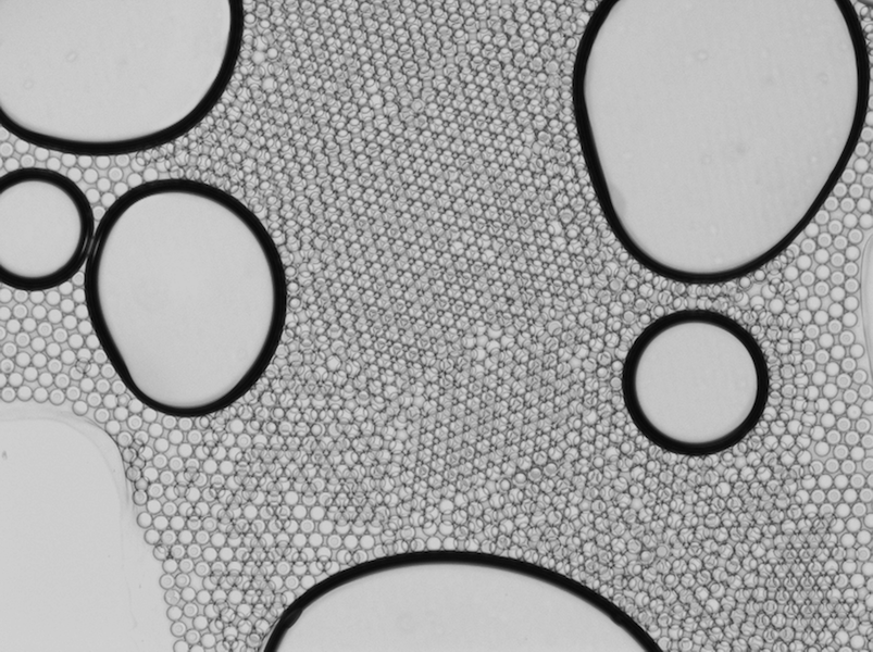
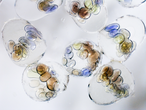
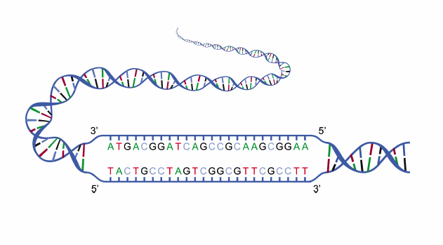
The figure above shows the principal difference between the two approaches for separated and dispersed multiphase flow models. In both exemplified cases, a function, Φ, is used to describe the presence of the gas and liquid phases. However, in the separated multiphase flow model, the different phases are exclusive, and there is a sharp phase boundary between them where the phase field function, Φ, changes abruptly. The phase field function does not have a physical meaning other than keeping track of the location of the phase boundaries.

In the dispersed multiphase flow model, the function Φ describes the local average volume fraction of gas, the dispersed phase, in the liquid, the continuous phase. The average volume fraction can smoothly find values between 0 and 1 everywhere in the domain, signifying if there are small or large amounts of bubbles in the otherwise homogenized domain. In other words, in the dispersed multiphase flow models, the gas and liquid phases can be defined in the same point in space and time, while in the separated multiphase flow models, there is either gas or liquid at a given point and time.

Separated Multiphase Flow Models

There are three different interface tracking methods in the COMSOL Multiphysics® software for separated multiphase flow models:

  • Level set
  • Phase field
  • Moving mesh

The level set and phase field methods are both field-based methods in which the interface between phases is represented as an isosurface of the level set or phase field functions. The moving mesh method is a completely different approach to the same problem. With this approach, the phase boundary is modeled as a geometrical surface separating two domains, with one phase on each side in the corresponding domains.

The field-based problems are usually solved on a fixed mesh. The moving mesh problems are obviously solved using a moving mesh.

The animation below shows the results from a model in which an emulsion is produced in a T-shaped microchannel, where the problem is solved with the phase field method. We can see in this animation that the phase boundary does not coincide with the faces and edges of the mesh. The phase boundary is represented by the isosurface of the phase field function.


The finite element mesh does not have to coincide with the phase boundary between two phases in the phase field and level set methods.

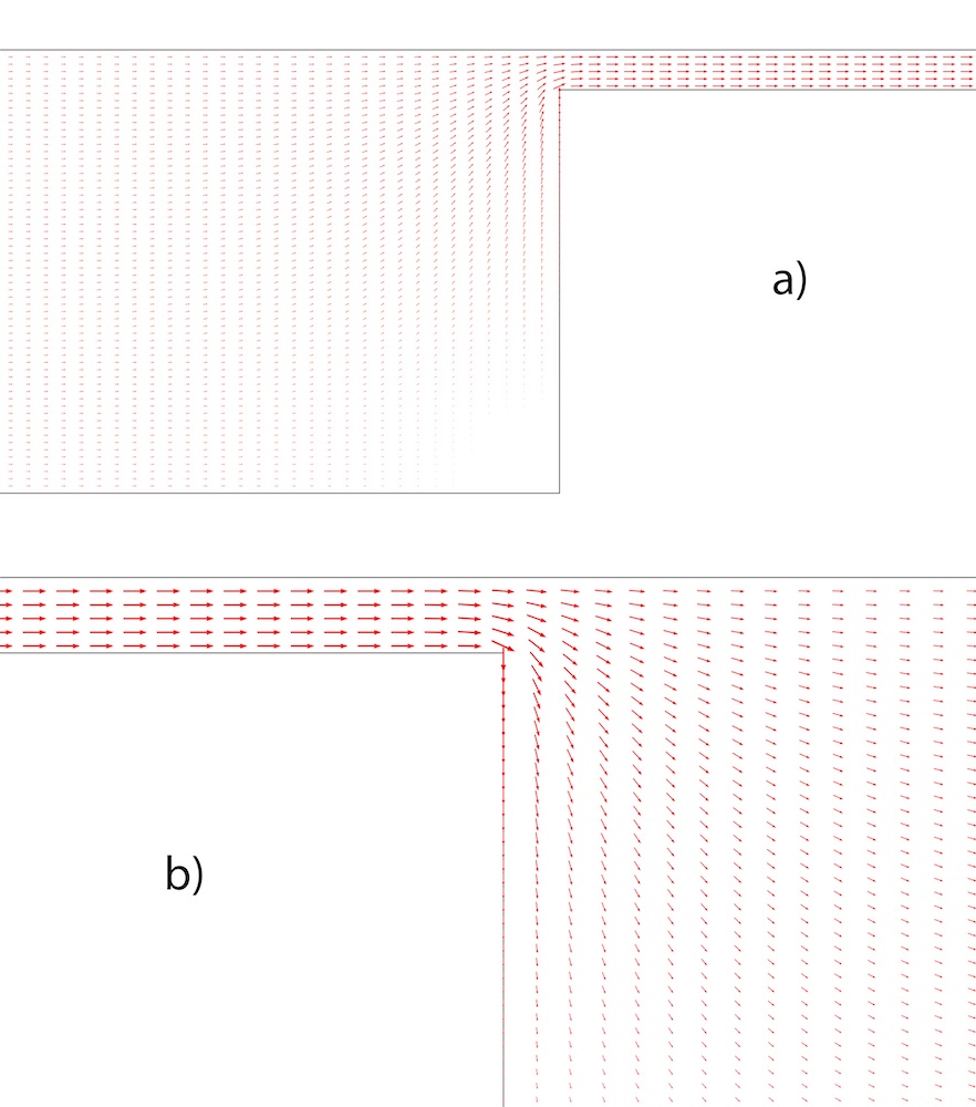
In contrast, the figure below shows the verification model of a rising bubble with moving mesh. The mesh follows the shape of the phase boundary and the edges coincide with this boundary. We can also see the drawback of the moving mesh model. The bubble deforms to such an extent that two secondary bubbles detach from the mother bubble. At this point, the original phase boundary has to be divided into several boundaries. The logic for that is not completely straightforward and this is not yet implemented in the COMSOL® software. Hence, the moving mesh method in the COMSOL® software cannot deal with topology changes. The phase field methods do not have this drawback and can handle any changes in shape of the phase boundary.


The rising bubble verification problem. A topology change occurs when two secondary bubbles break away from the mother bubble.

When Do We Use Field-Based Methods Vs. Moving Mesh?

Moving mesh methods allow for a higher accuracy for a given mesh. The fact that we can apply forces and fluxes directly on the phase boundary is an advantage in this respect. The field-based methods require a dense mesh around the interphase surface in order to resolve the isosurface that defines this surface. It is difficult to define an adaptive mesh that accurately follows the isosurface, which leads that the mesh usually has to be dense in a large volume around the isosurface. This lowers the performance of the field-based methods in relation to moving mesh for the same accuracy. So, when do we use the different methods?

  • For microfluidic systems where topology changes are not expected, then the moving mesh method is usually preferable
  • In cases where topology changes are expected, then a field-based method has to be used:
    • When the effects of surface tension are large, then the phase field method is the preferred method
    • When surface tension can be neglected, then the level set method is preferred

Separated Multiphase Flow Models and Turbulence Models

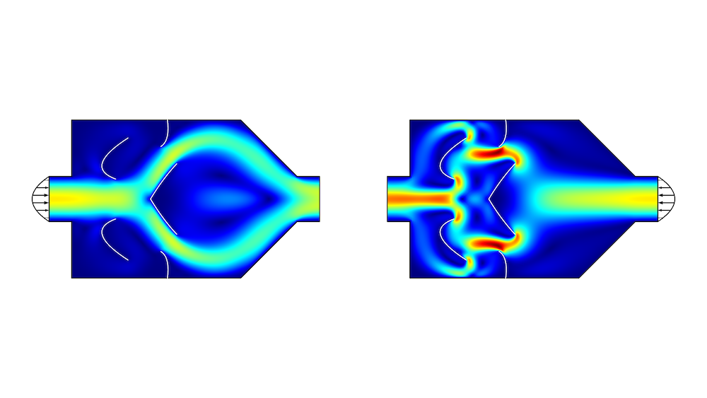
In cases where turbulence models are used, the details of the flow are lost, since only the mean velocity and pressure are resolved. With this in mind, effects of surface tension also become less important for the macroscopic description of the flow. Since turbulence also implies that the flow is relatively vigorous, also at the surface, it is almost impossible to avoid topology changes. Hence, for turbulent flow models and separated multiphase flow combinations, the level set method is preferred. Both the level set and phase field methods can be combined with all turbulence models in COMSOL Multiphysics, as seen in the figure and animation below.
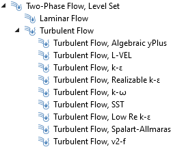
A screenshot showing a list of Two-Phase Flow, Level Set interfaces in COMSOL Multiphysics.
All turbulence models can be combined with the phase field and level set methods for two-phase flow in COMSOL Multiphysics.


Two-phase flow with water and air in a reactor modeled using the level set method in combination with the k-e turbulence model.

Dispersed Multiphase Flow Models

In cases where the phase boundaries cannot be resolved due to their complexity, dispersed multiphase flow models have to be used.

The CFD Module provides four different (in principle) models:

  • Bubbly flow model
    • For small volume fractions of a light phase in a denser phase
  • Mixture model
    • For a small volume fraction of a dispersed phase (or several dispersed phases) in a continuous phase that has about the same density as the dispersed phase or phases
  • Euler–Euler model
    • For any type of multiphase flow
    • Can handle any type of multiphase flow also dense particles in gases; for example, in fluidized beds
  • Euler–Lagrange models:
    • For a relatively small number (tens of thousands, not billions) of bubbles, droplets, or particles suspended in fluid
    • Each bubble, particle, droplet, or particle is modeled with an equation that defines the force balance of each particle in the fluid

When Do We Use the Different Dispersed Flow Multiphase Flow Models?

Bubbly Flow

The bubbly flow model is obviously used for gas bubbles in liquids. Since the momentum contribution from the dispersed phase is neglected, the model is only valid when the dispersed phase has a density that is several orders of magnitude smaller than the continuous phase.

Mixture

The mixture model is similar to the bubbly flow model, but it accounts for the momentum contribution of the dispersed phase. It is commonly used for modeling gas bubbles or solid particles dispersed in a liquid phase. The mixture model can also handle an arbitrary number of dispersed phases. Both the mixture model and the bubbly flow model assume that the dispersed phase is in equilibrium with the continuous phase; i.e., the dispersed phase cannot accelerate relative to the continuous phase. Hence, the mixture model cannot handle large solid particles dispersed in a gas.

Three side-by-side image showing different examples of modeling multiphase flow with the Mixture model.
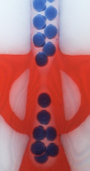
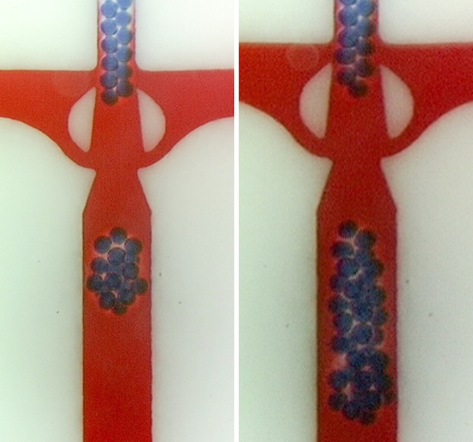
The mixture model used to model 5 different sizes of bubbles as the multiphase flow mixture is forced through an orifice. The shear in the flow causes larger bubbles to break up into smaller ones.

Euler–Euler

The Euler–Euler model is the most accurate dispersed multiphase flow model and also the most versatile. It can handle any type of dispersed multiphase flows. The dispersed phase is allowed to accelerate, and there is no real limit in the volume fractions for the different phases. However, it defines one set of Navier–Stokes equations for each phase.

In practice, the Euler–Euler model is only applicable for two-phase flow and even then, it is an expensive model with respect to computational cost (CPU time and memory). It is also relatively difficult to work with and requires good initial conditions to get convergence in the numerical solution.


Volume fraction of solid particles in a fluidized bed modeled using the Euler–Euler multiphase flow model.

Euler–Lagrange

When we have a few (tens of thousands but not billions) very small bubbles, droplets, or particles suspended in a continuous fluid, we may be able to use Euler–Lagrange models to simulate a multiphase flow system. These methods have the benefit of being relatively inexpensive, computation-wise. These models are usually also “nice” from a numerical point of view. They are therefore preferred when there is a relatively small number of particles of a dispersed phase in a continuous fluid.

Note that there are also methods to mimic a larger number of particles with Euler–Lagrange methods, using interaction terms and volume fractions that may mimic a system with billions of particles. These methods can be implemented in COMSOL Multiphysics, but they are not available in the predefined physics interfaces.
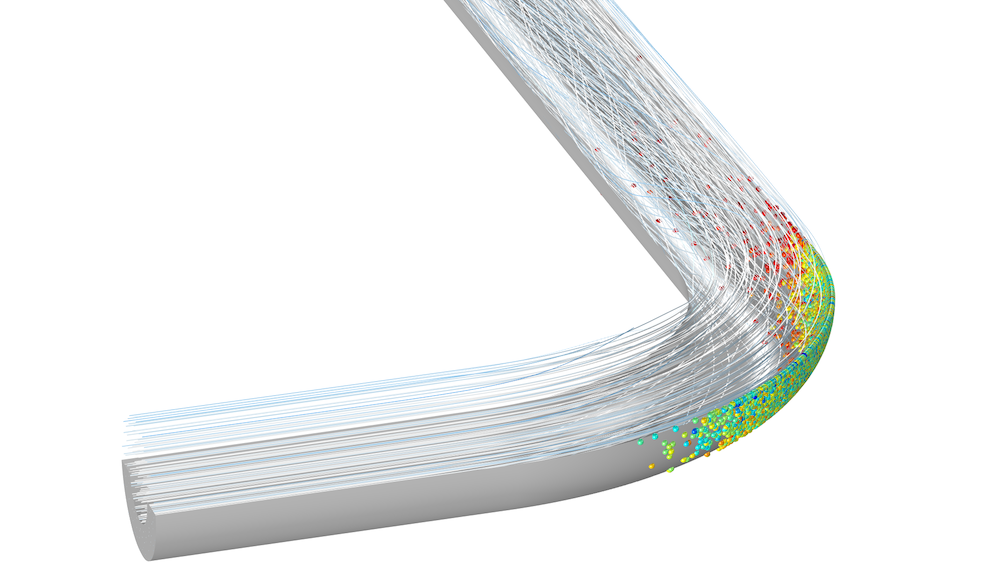
An image of a model showing particle flow in a pipe bend.
Euler–Lagrange multiphase flow models in COMSOL Multiphysics are available with the add-on CFD Module and Particle Tracing Module.

The mixture model is able to handle any combination of phases and is also computationally inexpensive. In most cases, it is advised that we start with this model, unless we deal with systems like fluidized beds (large particles with high density and high volume fractions of the dispersed phase), which can only be modeled with Euler–Euler models.

Dispersed Multiphase Flow Models and Turbulence

The dispersed multiphase flow models are approximative in their nature and fit very well with turbulence models, which are also approximative. It is possible to introduce interactions between dispersed phases and the continuous phase as well as between the bubbles, droplets, and particles in the dispersed phases. These interactions can have their origin in the turbulent eddies modeled with the turbulence model. The bubbly flow, mixture, and Euler–Lagrange multiphase flow models can be combined with all turbulence models in COMSOL Multiphysics. The Euler–Euler multiphase flow model is only predefined for the standard k-e turbulence models with realizability constraints.
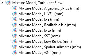
A screenshot of the interfaces for combining the Mixture model and turbulence models.
The mixture model can be combined with any turbulence model in COMSOL Multiphysics.

Concluding Remarks

Solving the numerical model equations for multiphase flow may be a very demanding task, even with access to supercomputers. If there were no computer power limitations, the surface tracking methods would be used for all types of mixtures. In reality, these models are limited to microfluidics and for the study of free surfaces of viscous liquids.

The dispersed multiphase flow methods allow for the studying of systems with millions and billions of bubbles, droplets, or particles. But even the simplest dispersed multiphase flow models can generate very complex and demanding model equations. The development of these models into variations that are well adapted to describe specific mixtures has allowed for engineers and scientists to study multiphase flow with a relatively good accuracy and with reasonable computational costs.

Stay tuned as we continue our discussion of multiphase flow simulation on the blog!

Exploring the 4 Basic Modes of Electrophoresis

$
0
0

DNA, RNA, proteins… All of these macromolecules can be analyzed using the electrokinetic process electrophoresis. In a 2020 webinar hosted by the American Institute of Chemical Engineers (AIChE), Professor Cornelius Ivory from Washington State University went over the four modes of electrophoresis: zone electrophoresis, moving-boundary electrophoresis, isotachophoresis, and isoelectric focusing — and discussed modeling them in the COMSOL Multiphysics® software. 

Electrophoresis Overview

Electrophoresis is a general term used to describe the movement of charged particles in a fluid under the influence of an electric field. The word itself is derived from Greek; electro referring to electricity and phoresis meaning “to carry” or “to bear”. 

One of the first observations of the electrokinetic process occurred over 200 years ago, in 1801, by French chemist Nicolas Gautherot. At the time, Gautherot saw electrophoresis taking place in a water droplet that was placed between two electrically attached metal plates (called electrodes).

Today, electrophoresis is commonly used to separate molecules based on their charge and size. This method can accurately separate macromolecules, such as DNA, RNA, proteins, nucleic acids, and plasmids. 

A simple schematic of the capillary electrophoresis (CE) process with parts labeled.
Sketch of capillary electrophoresis (CE). Image by Apblum. Licensed under CC BY-SA 3.0, via Wikimedia Commons. 

The diagram above shows capillary electrophoresis (CE) — a modern technique used to detect short tandem repeat alleles in forensic DNA laboratories

To get a comprehensive look at the mathematics behind electrophoresis, a good resource to start with is The Dynamics of Electrophoresis by Richard Mosher, Dudley Saville, and Wolfgang Thormann. 

The 4 Basic Modes of Electrophoresis

The four basic modes of electrophoresis are: 

  1. Zone electrophoresis
  2. Moving-boundary electrophoresis
  3. Isotachophoresis
  4. Isoelectric focusing

In most cases, the physics of new electrophoretic methods can be related back to these four modes.  

Zone Electrophoresis

Zone electrophoresis is often used by scientists to analyze biopolymers, nucleic acids, and proteins. This type of electrophoresis became widely used in the 1960s, thanks to the discovery of discontinuous buffers, and it is still the most popular mode in use today. 

Moving-Boundary Electrophoresis

Moving-boundary electrophoresis was developed in the 1930s by Swedish biochemist Arne Tiselius, who eventually went on to earn the Nobel Prize in Chemistry in 1948 for his work on electrophoresis and absorption analysis. This method is particularly beneficial when analyzing larger molecules, like proteins, which can be difficult to separate due to their differing charges. Historically, this method played an important role in moving the study of electrophoresis forward, but it isn’t widely applied today. 

Isotachophoresis

Isotachophoresis is based on moving-boundary electrophoresis, and it is a very powerful separation method. This technique has been around since the 1920s and is still widely applied in research today. For example, isotachophoresis is used in the analysis of organic acids in silage, anions in urine and serum, inorganic ions in water, proteins, and amino acids

Isoelectric Focusing

The fourth and final mode discussed in the AIChE webinar by Professor Ivory, isoelectric focusing, is often used in biological separations. In a previous blog post, we discussed how this type of electrophoresis is especially valued for its ability to concentrate and focus molecules into a fixed state

How are these four modes the same and how are they different?

Modeling Electrophoresis Using COMSOL Multiphysics®

In the AIChE webinar, Professor Ivory discussed how the bulk equations for modeling all modes of electrophoresis are always the same, but the initial conditions and boundary conditions vary from type to type. Ivory turned to COMSOL Multiphysics to model the four basic modes. 

Each model contains a cathodic reservoir, an anodic reservoir, and a channel; the cathodic and anodic reservoirs are described as boundary conditions, while the channel is the modeling domain. The initial conditions differ depending on which mode is used, and the models are all time-dependent, with the independent variables being the position in the channel and time.

In the table below, you can find the cathodic reservoir, anodic reservoir, and channel used for each mode. The governing equations in the channels are the Nernst–Planck equations in combination with the electroneutrality condition, for all four modes.

Mode Cathodic Reservoir  Anodic Reservoir  Channel
Zone electrophoresis Running buffer Running buffer Running buffer and sample (which should be dialyzed in practice)
Moving-boundary electrophoresis Sample Leading electrolyte  Leading electrolyte
Isotachophoresis Trailing electrolyte  Leading electrolyte  Trailing electrolyte, sample, and leading electrolyte
Isoelectric focusing Basic solution (high pH) Acidic solution (low pH) Carrier ampholytes and sample

For each model, Ivory accounts for seven dependent variables (ten for isoelectric focusing), including six chemical species (nine for isoelectric focusing) and the electric potential in the channel: 

  1. Sodium (Na)
  2. Chlorine (Cl)
  3. Tris (Tr)
  4. Acitate (Ac)
  5. Seperand 1 (Sp1)
  6. Seperand 2 (Sp2)
  7. Electric potential
  8. Two pseudo-ampholytes and tricine for isoelectric focusing

The different solutions’ pH in the channel is predefined, as a constant value or as a given pH profile (isoelectric focusing). In addition, each model requires the following input parameters and initial conditions:

  • Diffusion coefficients
  • Mobilities
  • Acid-base relationships
  • Reservoir concentrations
  • Operating voltages
  • Initial channel concentration profiles
  • Initial electric potential profile

Below, you can see each mode simulated in COMSOL Multiphysics. The plots show the concentration and pH in the channel at different given times after the sample enters the channel. We can here see the qualitatively different shapes of the sample profiles (red and blue).


Clockwise from top left: zone electrophoresis, moving-boundary electrophoresis, isoelectric focusing, and isotachophoresis.

Try It Yourself

Professor Ivory created 2 downloadable MPH-files for the electrophoresis models discussed above; one of the files focuses on zone electrophoresis modeling and the other contains complete models for all four basic modes of electrophoresis. 

You can find and download the files on the Application Exchange via the button below. Note that you must be logged into a COMSOL Access account with a valid software license to download the files.

How Does This Lip Gloss Appear to Defy Gravity?

$
0
0

In early 2020, a viral video showing an eye-catching lip gloss trick appeared on web browsers and phone screens around the world. The trick features lip gloss mysteriously flying into the air after being pulled from its tube-shaped container, making it look like the lip gloss defies gravity. After a little internet digging, we were able to find a lip gloss that performs the trick. To help further explain how this phenomenon occurs, we can turn to multiphysics simulation…

Explaining a Viral Trend with Simulation

Watch the “magic” lip gloss in action below, and then get an overview of what we think is causing this phenomenon. 


Continue reading to learn more about this captivating cosmetic…  

Finding a Gravity-Defying Lip Gloss

Acquiring the gravity-defying lip gloss was relatively easy. After testing out a handful of different glosses in a variety of shades and shines, we were able to get our hands on one that successfully and (consistently) demonstrates this trick. In order to prove that the gloss wasn’t just defective, we got four more of the same kind (a little excessive, but it’s in the name of science!) All five lip glosses demonstrate the exact same upward dripping effect.  


Tin Oxide: A Likely Culprit

Why do only certain lip glosses perform the gravity trick? A major reason has to do with the ingredients.

The average cosmetic contains anywhere from 15 to 50 ingredients.

After finding two different glosses that both consistently performed the floating phenomenon, we noticed they share a common ingredient: tin oxide. The Cosmetic Ingredient Review (CIR) defines tin oxide as an abrasive, bulking, and opacifying agent in cosmetics. The CIR also reports that tin oxide is safe to use in concentrations up to 1.3% in leave-on products. In its commercial form, it’s manufactured from tin metal by thermal oxidation.

A photograph of tin oxide in its mineral form, which supposedly makes lip gloss defy gravity.
Tin oxide in its mineral form cassiterite, or SnO2. Image in the public domain, via Wikimedia Commons.

Tin oxide is used in lip gloss because it adds a pearlescent shine, decreases density, and helps control viscosity. 

It’s important to note that tin oxide concentration isn’t the only reason why the glosses display the trick; it also has to do with their container sizes, applicator shapes, and other ingredients.

Investigating the Lip Gloss Phenomenon with Simulation

Our theory of why the lip gloss floats? The tin oxide particles inside the gloss’s container rub against each other due to velocity gradients and viscous effects, which creates friction. As the lip gloss’s applicator moves inside and is then separated from its container, the present friction causes a potential difference between the lip gloss in the container and the gloss on the applicator. Between the applicator and the container, an electric field is created. This field causes a driving force for the lip gloss on the applicator to fly toward the container, along the electric field lines (shown in the model below.)

The polarizations of the tin oxide (or SnO2 nanoparticles) is very high, which enhances the gloss’ dielectric behavior. (Dielectric materials are nonconductive, but they efficiently support electrostatic fields.) The gloss’ dielectric properties give a large-enough charge separation to continue the gravity-defying effect for several minutes.

Electrostatics in Dielectric Material

Considering that the lip gloss is dielectric in nature, let’s briefly go over electrostatics in dielectric materials at the microscopic level…

Electrostatics in idealized dielectric materials have bound charges, which can be replaced by an external electric field. This replacement results in induced electric dipoles within the dielectric material. These dipoles are pairs of positive and negative charges that in some way align with the electric field. The final result? An electric field forms inside the dielectric material (separate from that of free space). 

A recent study found that friction (like that caused by the tin oxide particles mixing together in the tube) can cause static electricity by bending the tiny protrusions on the surface of materials

Solving One Last Lip Gloss Mystery…

You might be wondering what happens to gloss that doesn’t make it back into its container. Unfortunately, it doesn’t magically disappear into the air. As the saying goes: What goes up must come down…

A photograph of lip gloss where some of the gloss spilled onto the table.

The gloss that didn’t make it back into the container fell onto the ground and the counter. 

Further Reading

See more examples of real-world phenomena explained using simulation in these blog posts:

Viewing all 31 articles
Browse latest View live


<script src="https://jsc.adskeeper.com/r/s/rssing.com.1596347.js" async> </script>